

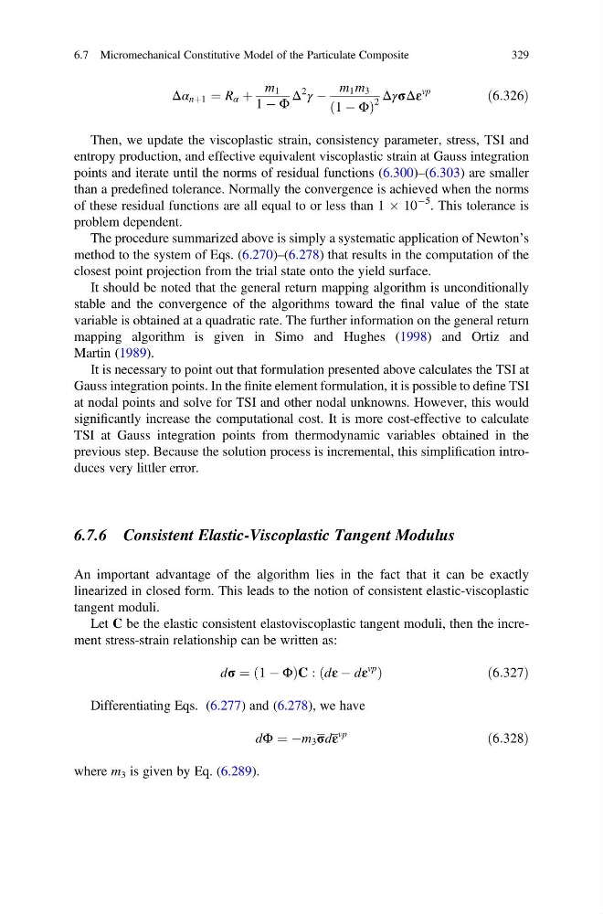
Δα nþ1 ¼ R α þ
m 1
1 À Φ
Δ
2
γ À
m 1 m 3
1 À Φ
ð
Þ
2
ΔγσΔε
vp
ð6:326Þ
Then, we update the viscoplastic strain, consistency parameter, stress, TSI and
entropy production, and effective equivalent viscoplastic strain at Gauss integration
points and iterate until the norms of residual functions (6.300)–(6.303) are smaller
than a predefined tolerance. Normally the convergence is achieved when the norms
of these residual functions are all equal to or less than 1 Â 10
À5 . This tolerance is
problem dependent.
The procedure summarized above is simply a systematic application of Newton’s
method to the system of Eqs. (6.270)–(6.278) that results in the computation of the
closest point projection from the trial state onto the yield surface.
It should be noted that the general return mapping algorithm is unconditionally
stable and the convergence of the algorithms toward the final value of the state
variable is obtained at a quadratic rate. The further information on the general return
mapping algorithm is given in Simo and Hughes (1998) and Ortiz and
Martin (1989).
It is necessary to point out that formulation presented above calculates the TSI at
Gauss integration points. In the finite element formulation, it is possible to define TSI
at nodal points and solve for TSI and other nodal unknowns. However, this would
significantly increase the computational cost. It is more cost-effective to calculate
TSI at Gauss integration points from thermodynamic variables obtained in the
previous step. Because the solution process is incremental, this simplification introduces very littler error.
6.7.6 Consistent Elastic-Viscoplastic Tangent Modulus
An important advantage of the algorithm lies in the fact that it can be exactly
linearized in closed form. This leads to the notion of consistent elastic-viscoplastic
tangent moduli.
Let C be the elastic consistent elastoviscoplastic tangent moduli, then the increment stress-strain relationship can be written as:
dσ ¼ 1 À Φ
ð
ÞC : dε À dε
vp
ð
Þ
ð 6:327Þ
Differentiating Eqs. (6.277) and (6.278), we have
dΦ ¼ Àm 3 σdε
vp
ð6:328Þ
where m 3 is given by Eq. (6.289).
6.7 Micromechanical Constitutive Model of the Particulate Composite
329
m 1
1 À Φ
Δ
2
γ À
m 1 m 3
1 À Φ
ð
Þ
2
ΔγσΔε
vp
ð6:326Þ
Then, we update the viscoplastic strain, consistency parameter, stress, TSI and
entropy production, and effective equivalent viscoplastic strain at Gauss integration
points and iterate until the norms of residual functions (6.300)–(6.303) are smaller
than a predefined tolerance. Normally the convergence is achieved when the norms
of these residual functions are all equal to or less than 1 Â 10
À5 . This tolerance is
problem dependent.
The procedure summarized above is simply a systematic application of Newton’s
method to the system of Eqs. (6.270)–(6.278) that results in the computation of the
closest point projection from the trial state onto the yield surface.
It should be noted that the general return mapping algorithm is unconditionally
stable and the convergence of the algorithms toward the final value of the state
variable is obtained at a quadratic rate. The further information on the general return
mapping algorithm is given in Simo and Hughes (1998) and Ortiz and
Martin (1989).
It is necessary to point out that formulation presented above calculates the TSI at
Gauss integration points. In the finite element formulation, it is possible to define TSI
at nodal points and solve for TSI and other nodal unknowns. However, this would
significantly increase the computational cost. It is more cost-effective to calculate
TSI at Gauss integration points from thermodynamic variables obtained in the
previous step. Because the solution process is incremental, this simplification introduces very littler error.
6.7.6 Consistent Elastic-Viscoplastic Tangent Modulus
An important advantage of the algorithm lies in the fact that it can be exactly
linearized in closed form. This leads to the notion of consistent elastic-viscoplastic
tangent moduli.
Let C be the elastic consistent elastoviscoplastic tangent moduli, then the increment stress-strain relationship can be written as:
dσ ¼ 1 À Φ
ð
ÞC : dε À dε
vp
ð
Þ
ð 6:327Þ
Differentiating Eqs. (6.277) and (6.278), we have
dΦ ¼ Àm 3 σdε
vp
ð6:328Þ
where m 3 is given by Eq. (6.289).
6.7 Micromechanical Constitutive Model of the Particulate Composite
329