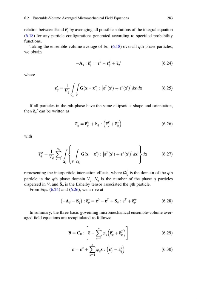
relation between ε and ε
Ã
q by averaging all possible solutions of the integral equation
(6.18) for any particle configurations generated according to specified probability
functions.
Taking the ensemble-volume average of Eq. (6.18) over all qth-phase particles,
we obtain
ÀA q : ε
Ã
q ¼ ε
0
À ε
T
q þ ε q
0
ð6:24Þ
where
ε
0
q ¼
1
V q
Z
V q
Z
V
G x 2 x
0
ð
Þ: ε
T x
0
ð Þ þ ε
à x
0
ð Þ
Â
Ã
dx
0 dx
ð6:25Þ
If all particles in the qth-phase have the same ellipsoidal shape and orientation,
then ε q
0 can be written as
ε
0
q ¼ ε
0p
q þ S q : ε
T
q þ ε
Ã
q
ð6:26Þ
with
ε
0p
q ¼
1
V q
X N q
i¼1
Z
Ω
i
q
Z
VÀΩ
i
q
G x 2 x
0
ð
Þ: ε
T x
0
ð Þ þ ε
à x
0
ð Þ
Â
Ã
dx
0
8
> <
> :
9
> =
> ;
dx
ð6:27Þ
representing the interparticle interaction effects, where Ω
i
q is the domain of the qth
particle in the qth phase domain V q , N q is the number of the phase q particles
dispersed in V, and S q is the Eshelby tensor associated the qth particle.
From Eqs. (6.24) and (6.26), we arrive at
ÀA q À S q
À
Á : ε
Ã
q ¼ ε
0
À ε
T
þ S q : ε
T
þ ε
0p
q
ð6:28Þ
In summary, the three basic governing micromechanical ensemble-volume averaged field equations are recapitulated as follows:
σ ¼ C 0 : ε À
X n
q¼1
φ q ε
Ã
q þ ε
T
q
"
#
ð6:29Þ
ε ¼ ε
0
þ
X n
q¼1
φ q s : ε
T
q þ ε
Ã
q
ð6:30Þ
6.2 Ensemble-Volume Averaged Micromechanical Field Equations
283