

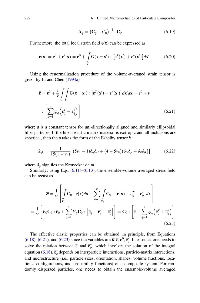
A q ¼ C q À C 0
À
Á À1 Á C 0
ð6:19Þ
Furthermore, the total local strain field ε(x) can be expressed as
ε x
ð Þ ¼ ε
0
þ ε
0 x
ð Þ ¼ ε
0
þ
Z
V
G x 2 x
0
ð
Þ: ε
T x
0
ð Þ þ ε
à x
0
ð Þ
Â
Ã
dx
0
ð6:20Þ
Using the renormalization procedure of the volume-averaged strain tensor is
given by Ju and Chen (1994a)
ε ¼ ε
0
þ
1
V
Z
V
Z
V
G x 2 x
0
ð
Þ: ε
T x
0
ð Þ þ ε
à x
0
ð Þ
Â
Ã
dx
0 dx ¼ ε
0
þ s
:
X n
q¼1
φ q ε
T
q þ ε
Ã
q
"
#
ð6:21Þ
where s is a constant tensor for uni-directionally aligned and similarly ellipsoidal
filler particles. If the linear elastic matrix material is isotropic and all inclusions are
spherical, then the s takes the form of the Eshelby tensor S:
S ijkl ¼
1
15 1 À v 0
ð
Þ
5v 0 À 1
ð
Þ δ ij δ kl þ 4 À 5v 0
ð
Þ δ ik δ jl þ δ il δ jk
À
Á
Â
Ã
ð6:22Þ
where δ ij signifies the Kronecker delta.
Similarly, using Eqs. (6.11)–(6.13), the ensemble-volume averaged stress field
can be recast as
σ ¼
1
V
Z
V 0
C 0 : ε x
ð Þdx þ
X n
q¼1
Z
V q
C 0 : ε x
ð Þ À ε
T
q À ε
Ã
q
h
i
dx
2
6
4
3
7
5
¼
1
V
V 0 C 0 : ε 0 þ
X n
q¼1
V q C 0 : ε q À ε
T
q À ε
Ã
q
h
i
"
#
¼ C 0 : ε À
X n
q¼1
φ q ε
T
q þ ε
Ã
q
"
#
ð6:23Þ
The effective elastic properties can be obtained, in principle, from Equations
(6.18), (6.21), and (6.23) since the variables are σ, ε, ε
0 , ε
Ã
q . In essence, one needs to
solve the relation between ε and ε
Ã
q , which involves the solution of the integral
equation (6.18). ε
Ã
q depends on interparticle interactions, particle-matrix interactions,
and microstructure (i.e., particle sizes, orientation, shapes, volume fractions, locations, configurations, and probability functions) of a composite system. For randomly dispersed particles, one needs to obtain the ensemble-volume averaged
282
6 Unified Micromechanics of Particulate Composites
À
Á À1 Á C 0
ð6:19Þ
Furthermore, the total local strain field ε(x) can be expressed as
ε x
ð Þ ¼ ε
0
þ ε
0 x
ð Þ ¼ ε
0
þ
Z
V
G x 2 x
0
ð
Þ: ε
T x
0
ð Þ þ ε
à x
0
ð Þ
Â
Ã
dx
0
ð6:20Þ
Using the renormalization procedure of the volume-averaged strain tensor is
given by Ju and Chen (1994a)
ε ¼ ε
0
þ
1
V
Z
V
Z
V
G x 2 x
0
ð
Þ: ε
T x
0
ð Þ þ ε
à x
0
ð Þ
Â
Ã
dx
0 dx ¼ ε
0
þ s
:
X n
q¼1
φ q ε
T
q þ ε
Ã
q
"
#
ð6:21Þ
where s is a constant tensor for uni-directionally aligned and similarly ellipsoidal
filler particles. If the linear elastic matrix material is isotropic and all inclusions are
spherical, then the s takes the form of the Eshelby tensor S:
S ijkl ¼
1
15 1 À v 0
ð
Þ
5v 0 À 1
ð
Þ δ ij δ kl þ 4 À 5v 0
ð
Þ δ ik δ jl þ δ il δ jk
À
Á
Â
Ã
ð6:22Þ
where δ ij signifies the Kronecker delta.
Similarly, using Eqs. (6.11)–(6.13), the ensemble-volume averaged stress field
can be recast as
σ ¼
1
V
Z
V 0
C 0 : ε x
ð Þdx þ
X n
q¼1
Z
V q
C 0 : ε x
ð Þ À ε
T
q À ε
Ã
q
h
i
dx
2
6
4
3
7
5
¼
1
V
V 0 C 0 : ε 0 þ
X n
q¼1
V q C 0 : ε q À ε
T
q À ε
Ã
q
h
i
"
#
¼ C 0 : ε À
X n
q¼1
φ q ε
T
q þ ε
Ã
q
"
#
ð6:23Þ
The effective elastic properties can be obtained, in principle, from Equations
(6.18), (6.21), and (6.23) since the variables are σ, ε, ε
0 , ε
Ã
q . In essence, one needs to
solve the relation between ε and ε
Ã
q , which involves the solution of the integral
equation (6.18). ε
Ã
q depends on interparticle interactions, particle-matrix interactions,
and microstructure (i.e., particle sizes, orientation, shapes, volume fractions, locations, configurations, and probability functions) of a composite system. For randomly dispersed particles, one needs to obtain the ensemble-volume averaged
282
6 Unified Micromechanics of Particulate Composites