

radial return and return mapping scheme is presented. The next and final step treats
the full damaged rate-dependent case and presents the return mapping algorithm
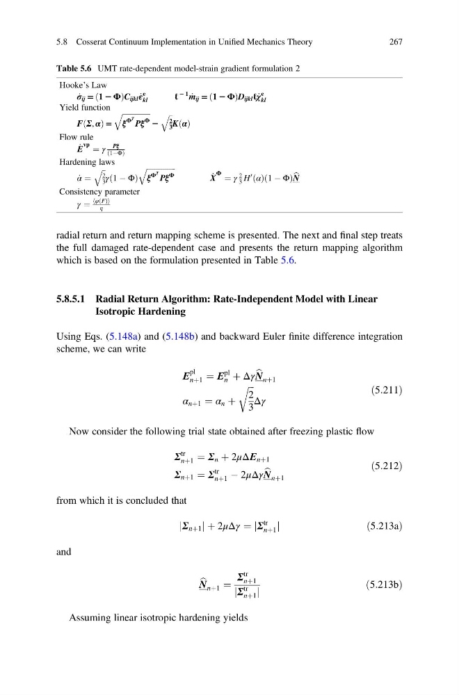
which is based on the formulation presented in Table 5.6.
5.8.5.1 Radial Return Algorithm: Rate-Independent Model with Linear
Isotropic Hardening
Using Eqs. (5.148a) and (5.148b) and backward Euler finite difference integration
scheme, we can write
Ε
pl
nþ1 ¼ Ε
pl
n þ Δγ b
N nþ1
α nþ1 ¼ α n þ
ffiffi ffi
2
3
r
Δγ
ð5:211Þ
Now consider the following trial state obtained after freezing plastic flow
Σ
tr
nþ1 ¼ Σ n þ 2μΔΕ nþ1
Σ nþ1 ¼ Σ
tr
nþ1 À 2μΔγ b
N nþ1
ð5:212Þ
from which it is concluded that
jΣ nþ1 j þ 2μΔγ ¼ jΣ
tr
nþ1 j
ð 5:213aÞ
and
b
N nþ1 ¼
Σ
tr
nþ1
jΣ
tr
nþ1 j
ð5:213bÞ
Assuming linear isotropic hardening yields
Table 5.6 UMT rate-dependent model-strain gradient formulation 2
Hooke’s Law
_
σ ij = 1 2 Φ
ð
ÞC ijkl _
ε
e
kl
ℓ
2 1 _
m ij = 1 2 Φ
ð
ÞD ijkl ℓ _
χ
e
kl
Yield function
F Σ, α
ð
Þ=
ffiffiffiffiffiffiffiffiffiffiffiffiffiffiffi ffi
ξ
Φ
T
Pξ
Φ
q
2
ffiffi
2
3
q
K α
ð Þ
Flow rule
_
Ε
vp ¼ γ
Pξ
1ÀΦ
ð
Þ
Hardening laws
_
α ¼
ffiffi
2
3
q
γ 1 À Φ
ð
Þ
ffiffiffiffiffiffiffiffiffiffiffiffiffiffiffi ffi
ξ
Φ
T
Pξ
Φ
q
_
X
Φ ¼ γ
2
3 H
0 α
ð Þ 1 À Φ
ð
Þ b
N
Consistency parameter
γ ¼
φ F
ð Þ
h
i
η
5.8 Cosserat Continuum Implementation in Unified Mechanics Theory
267
the full damaged rate-dependent case and presents the return mapping algorithm
which is based on the formulation presented in Table 5.6.
5.8.5.1 Radial Return Algorithm: Rate-Independent Model with Linear
Isotropic Hardening
Using Eqs. (5.148a) and (5.148b) and backward Euler finite difference integration
scheme, we can write
Ε
pl
nþ1 ¼ Ε
pl
n þ Δγ b
N nþ1
α nþ1 ¼ α n þ
ffiffi ffi
2
3
r
Δγ
ð5:211Þ
Now consider the following trial state obtained after freezing plastic flow
Σ
tr
nþ1 ¼ Σ n þ 2μΔΕ nþ1
Σ nþ1 ¼ Σ
tr
nþ1 À 2μΔγ b
N nþ1
ð5:212Þ
from which it is concluded that
jΣ nþ1 j þ 2μΔγ ¼ jΣ
tr
nþ1 j
ð 5:213aÞ
and
b
N nþ1 ¼
Σ
tr
nþ1
jΣ
tr
nþ1 j
ð5:213bÞ
Assuming linear isotropic hardening yields
Table 5.6 UMT rate-dependent model-strain gradient formulation 2
Hooke’s Law
_
σ ij = 1 2 Φ
ð
ÞC ijkl _
ε
e
kl
ℓ
2 1 _
m ij = 1 2 Φ
ð
ÞD ijkl ℓ _
χ
e
kl
Yield function
F Σ, α
ð
Þ=
ffiffiffiffiffiffiffiffiffiffiffiffiffiffiffi ffi
ξ
Φ
T
Pξ
Φ
q
2
ffiffi
2
3
q
K α
ð Þ
Flow rule
_
Ε
vp ¼ γ
Pξ
1ÀΦ
ð
Þ
Hardening laws
_
α ¼
ffiffi
2
3
q
γ 1 À Φ
ð
Þ
ffiffiffiffiffiffiffiffiffiffiffiffiffiffiffi ffi
ξ
Φ
T
Pξ
Φ
q
_
X
Φ ¼ γ
2
3 H
0 α
ð Þ 1 À Φ
ð
Þ b
N
Consistency parameter
γ ¼
φ F
ð Þ
h
i
η
5.8 Cosserat Continuum Implementation in Unified Mechanics Theory
267