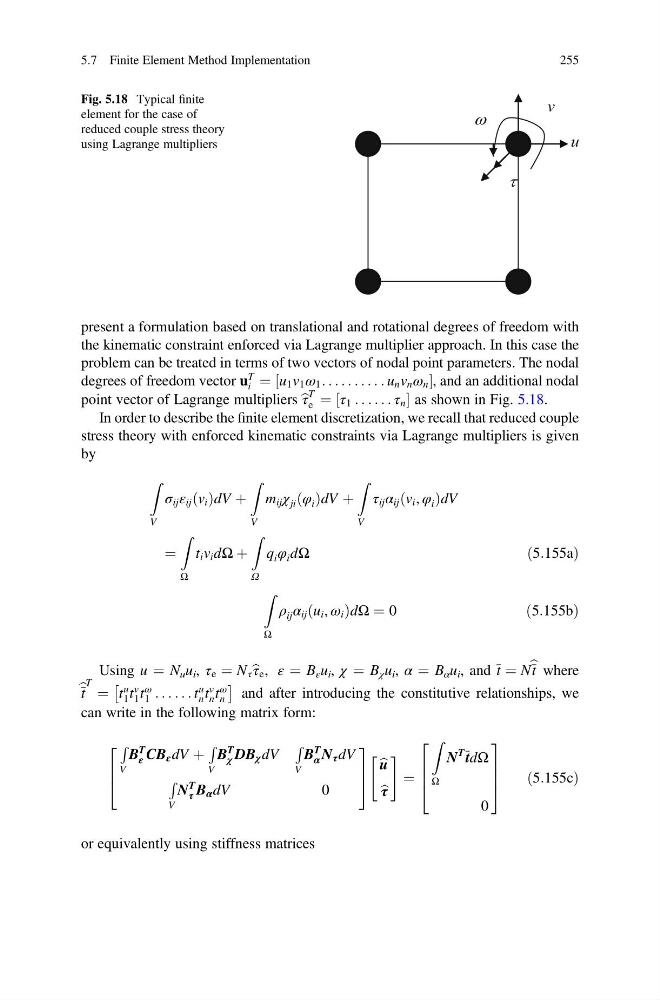
present a formulation based on translational and rotational degrees of freedom with
the kinematic constraint enforced via Lagrange multiplier approach. In this case the
problem can be treated in terms of two vectors of nodal point parameters. The nodal
degrees of freedom vector u
T
i ¼ u 1 v 1 ω 1 : . . . . . . . . . u n v n ω n
½
Š , and an additional nodal
point vector of Lagrange multipliers b τ
T
e ¼ τ 1 . . . . . . τ n
½
Šas shown in Fig. 5.18.
In order to describe the finite element discretization, we recall that reduced couple
stress theory with enforced kinematic constraints via Lagrange multipliers is given
by
Z
V
σ ij ε ij v i
ð ÞdV þ
Z
V
m ij χ ji φ i
ð ÞdV þ
Z
V
τ ij α ij v i , φ i
ð
ÞdV
¼
Z
Ω
t i v i dΩ þ
Z
Ω
q i φ i dΩ
ð5:155aÞ
Z
Ω
ρ ij α ij u i , ω i
ð
ÞdΩ ¼ 0
ð5:155bÞ
Using u ¼ N u u i , τ e ¼ N τ b τ e , ε ¼ B ε u i , χ ¼ B χ u i , α ¼ B α u i , and t ¼ N b t where
b t
T ¼ t
u
1 t
v
1 t
ω
1 . . . . . . t
u
n t
v
n t
ω
n
Â
Ã
and after introducing the constitutive relationships, we
can write in the following matrix form:
R
V
B
T
ε CB ε dV þ
R
V
B
T
χ DB χ dV
R
V
B
T
α N τ dV
R
V
N
T
τ B α dV
0
2
6
4
3
7
5
b u
b τ
" #
¼
Z
Ω
N
T tdΩ
0
2
6
6
4
3
7
7
5
ð5:155cÞ
or equivalently using stiffness matrices
v
u
ω
τ
Fig. 5.18 Typical finite
element for the case of
reduced couple stress theory
using Lagrange multipliers
5.7 Finite Element Method Implementation
255