implies that elements with C
1 continuity are needed to satisfy displacement compatibility requirements. Assuming that such an element is readily available, the nodal
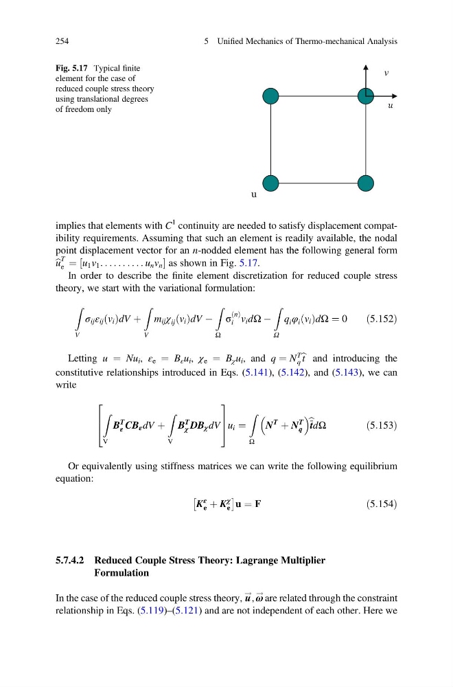
point displacement vector for an n-nodded element has the following general form
b u
T
e ¼ u 1 v 1 : . . . . . . . . . u n v n
½
Š as shown in Fig. 5.17.
In order to describe the finite element discretization for reduced couple stress
theory, we start with the variational formulation:
Z
V
σ ij ε ij v i
ð ÞdV þ
Z
V
m ij χ ij v i
ð ÞdV À
Z
Ω
σ
n
ð Þ
i v i dΩ À
Z
Ω
q i φ i v i
ð ÞdΩ ¼ 0
ð5:152Þ
Letting u ¼ Nu i , ε e ¼ B ε u i , χ e ¼ B χ u i , and q ¼ N
T
q
b t and introducing the
constitutive relationships introduced in Eqs. (5.141), (5.142), and (5.143), we can
write
Z
V
B
T
ε CB ε dV þ
Z
V
B
T
χ DB χ dV
2
6
4
3
7
5ui ¼
Z
Ω
N
T
þ N
T
q
b tdΩ
ð5:153Þ
Or equivalently using stiffness matrices we can write the following equilibrium
equation:
K
ε
e þ K
χ
e
Â
Ã
u ¼ F
ð5:154Þ
5.7.4.2 Reduced Couple Stress Theory: Lagrange Multiplier
Formulation
In the case of the reduced couple stress theory, u
!
, ω
! are related through the constraint
relationship in Eqs. (5.119)–(5.121) and are not independent of each other. Here we
u
v
Fig. 5.17 Typical finite
element for the case of
reduced couple stress theory
using translational degrees
of freedom only
254
5 Unified Mechanics of Thermo-mechanical Analysis