

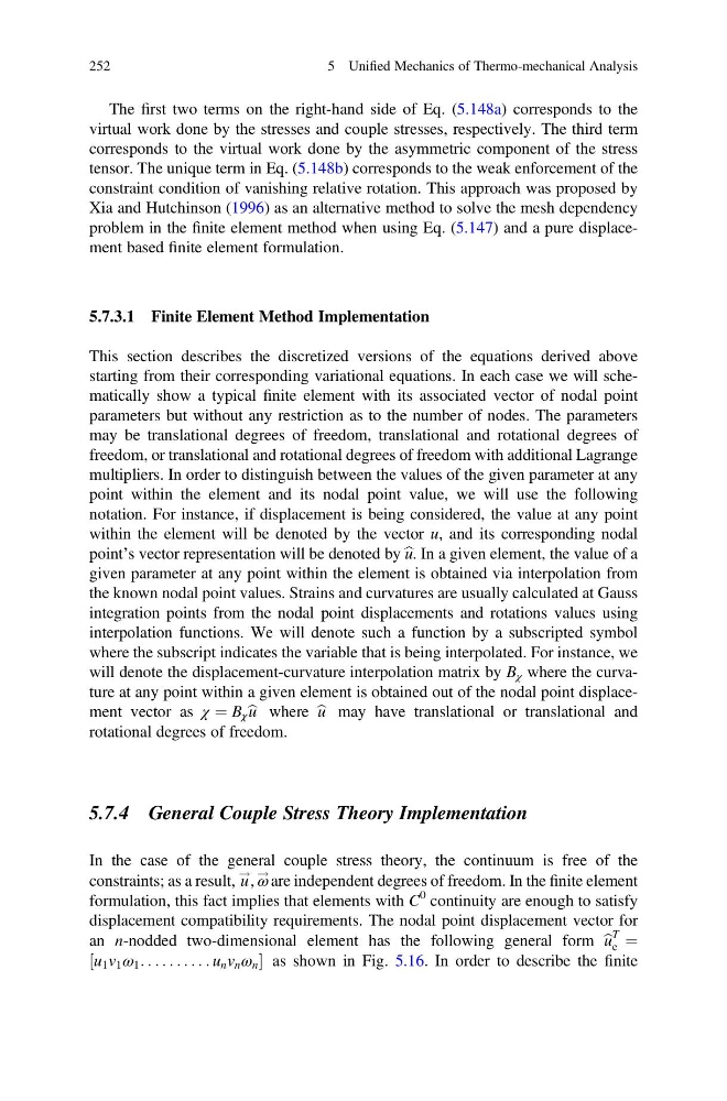
The first two terms on the right-hand side of Eq. (5.148a) corresponds to the
virtual work done by the stresses and couple stresses, respectively. The third term
corresponds to the virtual work done by the asymmetric component of the stress
tensor. The unique term in Eq. (5.148b) corresponds to the weak enforcement of the
constraint condition of vanishing relative rotation. This approach was proposed by
Xia and Hutchinson (1996) as an alternative method to solve the mesh dependency
problem in the finite element method when using Eq. (5.147) and a pure displacement based finite element formulation.
5.7.3.1 Finite Element Method Implementation
This section describes the discretized versions of the equations derived above
starting from their corresponding variational equations. In each case we will schematically show a typical finite element with its associated vector of nodal point
parameters but without any restriction as to the number of nodes. The parameters
may be translational degrees of freedom, translational and rotational degrees of
freedom, or translational and rotational degrees of freedom with additional Lagrange
multipliers. In order to distinguish between the values of the given parameter at any
point within the element and its nodal point value, we will use the following
notation. For instance, if displacement is being considered, the value at any point
within the element will be denoted by the vector u, and its corresponding nodal
point’s vector representation will be denoted by b u. In a given element, the value of a
given parameter at any point within the element is obtained via interpolation from
the known nodal point values. Strains and curvatures are usually calculated at Gauss
integration points from the nodal point displacements and rotations values using
interpolation functions. We will denote such a function by a subscripted symbol
where the subscript indicates the variable that is being interpolated. For instance, we
will denote the displacement-curvature interpolation matrix by B χ where the curvature at any point within a given element is obtained out of the nodal point displacement vector as χ ¼ B χ b u where b u may have translational or translational and
rotational degrees of freedom.
5.7.4 General Couple Stress Theory Implementation
In the case of the general couple stress theory, the continuum is free of the
constraints; as a result, u
!
, ω
! are independent degrees of freedom. In the finite element
formulation, this fact implies that elements with C
0 continuity are enough to satisfy
displacement compatibility requirements. The nodal point displacement vector for
an n-nodded two-dimensional element has the following general form b u
T
e ¼
u 1 v 1 ω 1 : . . . . . . . . . u n v n ω n
½
as shown in Fig. 5.16. In order to describe the finite
252
5 Unified Mechanics of Thermo-mechanical Analysis
virtual work done by the stresses and couple stresses, respectively. The third term
corresponds to the virtual work done by the asymmetric component of the stress
tensor. The unique term in Eq. (5.148b) corresponds to the weak enforcement of the
constraint condition of vanishing relative rotation. This approach was proposed by
Xia and Hutchinson (1996) as an alternative method to solve the mesh dependency
problem in the finite element method when using Eq. (5.147) and a pure displacement based finite element formulation.
5.7.3.1 Finite Element Method Implementation
This section describes the discretized versions of the equations derived above
starting from their corresponding variational equations. In each case we will schematically show a typical finite element with its associated vector of nodal point
parameters but without any restriction as to the number of nodes. The parameters
may be translational degrees of freedom, translational and rotational degrees of
freedom, or translational and rotational degrees of freedom with additional Lagrange
multipliers. In order to distinguish between the values of the given parameter at any
point within the element and its nodal point value, we will use the following
notation. For instance, if displacement is being considered, the value at any point
within the element will be denoted by the vector u, and its corresponding nodal
point’s vector representation will be denoted by b u. In a given element, the value of a
given parameter at any point within the element is obtained via interpolation from
the known nodal point values. Strains and curvatures are usually calculated at Gauss
integration points from the nodal point displacements and rotations values using
interpolation functions. We will denote such a function by a subscripted symbol
where the subscript indicates the variable that is being interpolated. For instance, we
will denote the displacement-curvature interpolation matrix by B χ where the curvature at any point within a given element is obtained out of the nodal point displacement vector as χ ¼ B χ b u where b u may have translational or translational and
rotational degrees of freedom.
5.7.4 General Couple Stress Theory Implementation
In the case of the general couple stress theory, the continuum is free of the
constraints; as a result, u
!
, ω
! are independent degrees of freedom. In the finite element
formulation, this fact implies that elements with C
0 continuity are enough to satisfy
displacement compatibility requirements. The nodal point displacement vector for
an n-nodded two-dimensional element has the following general form b u
T
e ¼
u 1 v 1 ω 1 : . . . . . . . . . u n v n ω n
½
as shown in Fig. 5.16. In order to describe the finite
252
5 Unified Mechanics of Thermo-mechanical Analysis