

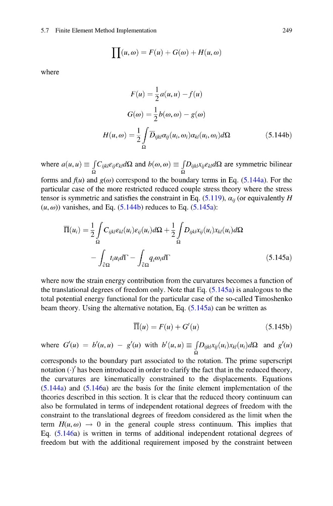
Y
u, ω
ð
Þ ¼ F u
ð Þ þ G ω
ð Þ þ H u, ω
ð
Þ
where
F u
ð Þ ¼
1
2
a u, u
ð ÞÀf u
ð Þ
G ω
ð Þ ¼
1
2
b ω, ω
ð
ÞÀg ω
ð Þ
H u, ω
ð
Þ ¼
1
2
Z
Ω
D ijkl α ij u i , ω i
ð
Þα kl u i , ω i
ð
ÞdΩ
ð5:144bÞ
where a u, u
ð Þ
R
Ω
C ijkl ε ij ε kl dΩ and b ω, ω
ð
Þ
R
Ω
D ijkl x ij ε kl dΩ are symmetric bilinear
forms and f(u) and g(ω) correspond to the boundary terms in Eq. (5.144a). For the
particular case of the more restricted reduced couple stress theory where the stress
tensor is symmetric and satisfies the constraint in Eq. (5.119), α ij (or equivalently H
(u, ω)) vanishes, and Eq. (5.144b) reduces to Eq. (5.145a):
Π u i
ð Þ ¼
1
2
Z
Ω
C ijkl ε kl u i
ð Þε ij u i
ð ÞdΩ þ
1
2
Z
Ω
D ijkl x ij u i
ð Þx kl u i
ð ÞdΩ
À
Z
∂Ω
t i u i dΓ À
Z
∂Ω
q i ω i dΓ
ð5:145aÞ
where now the strain energy contribution from the curvatures becomes a function of
the translational degrees of freedom only. Note that Eq. (5.145a) is analogous to the
total potential energy functional for the particular case of the so-called Timoshenko
beam theory. Using the alternative notation, Eq. (5.145a) can be written as
Π u
ð Þ ¼ F u
ð Þ þ G
0 u
ð Þ
ð5:145bÞ
where G
0
(u) ¼ b
0 (u, u) À g
0 (u) with b
0 u, u
ð Þ
R
Ω
D ijkl x ij u i
ð Þx kl u i
ð ÞdΩ and g
0 (u)
corresponds to the boundary part associated to the rotation. The prime superscript
notation (Á)
0 has been introduced in order to clarify the fact that in the reduced theory,
the curvatures are kinematically constrained to the displacements. Equations
(5.144a) and (5.146a) are the basis for the finite element implementation of the
theories described in this section. It is clear that the reduced theory continuum can
also be formulated in terms of independent rotational degrees of freedom with the
constraint to the translational degrees of freedom considered as the limit when the
term H(u, ω) ! 0 in the general couple stress continuum. This implies that
Eq. (5.146a) is written in terms of additional independent rotational degrees of
freedom but with the additional requirement imposed by the constraint between
5.7 Finite Element Method Implementation
249
u, ω
ð
Þ ¼ F u
ð Þ þ G ω
ð Þ þ H u, ω
ð
Þ
where
F u
ð Þ ¼
1
2
a u, u
ð ÞÀf u
ð Þ
G ω
ð Þ ¼
1
2
b ω, ω
ð
ÞÀg ω
ð Þ
H u, ω
ð
Þ ¼
1
2
Z
Ω
D ijkl α ij u i , ω i
ð
Þα kl u i , ω i
ð
ÞdΩ
ð5:144bÞ
where a u, u
ð Þ
R
Ω
C ijkl ε ij ε kl dΩ and b ω, ω
ð
Þ
R
Ω
D ijkl x ij ε kl dΩ are symmetric bilinear
forms and f(u) and g(ω) correspond to the boundary terms in Eq. (5.144a). For the
particular case of the more restricted reduced couple stress theory where the stress
tensor is symmetric and satisfies the constraint in Eq. (5.119), α ij (or equivalently H
(u, ω)) vanishes, and Eq. (5.144b) reduces to Eq. (5.145a):
Π u i
ð Þ ¼
1
2
Z
Ω
C ijkl ε kl u i
ð Þε ij u i
ð ÞdΩ þ
1
2
Z
Ω
D ijkl x ij u i
ð Þx kl u i
ð ÞdΩ
À
Z
∂Ω
t i u i dΓ À
Z
∂Ω
q i ω i dΓ
ð5:145aÞ
where now the strain energy contribution from the curvatures becomes a function of
the translational degrees of freedom only. Note that Eq. (5.145a) is analogous to the
total potential energy functional for the particular case of the so-called Timoshenko
beam theory. Using the alternative notation, Eq. (5.145a) can be written as
Π u
ð Þ ¼ F u
ð Þ þ G
0 u
ð Þ
ð5:145bÞ
where G
0
(u) ¼ b
0 (u, u) À g
0 (u) with b
0 u, u
ð Þ
R
Ω
D ijkl x ij u i
ð Þx kl u i
ð ÞdΩ and g
0 (u)
corresponds to the boundary part associated to the rotation. The prime superscript
notation (Á)
0 has been introduced in order to clarify the fact that in the reduced theory,
the curvatures are kinematically constrained to the displacements. Equations
(5.144a) and (5.146a) are the basis for the finite element implementation of the
theories described in this section. It is clear that the reduced theory continuum can
also be formulated in terms of independent rotational degrees of freedom with the
constraint to the translational degrees of freedom considered as the limit when the
term H(u, ω) ! 0 in the general couple stress continuum. This implies that
Eq. (5.146a) is written in terms of additional independent rotational degrees of
freedom but with the additional requirement imposed by the constraint between
5.7 Finite Element Method Implementation
249