

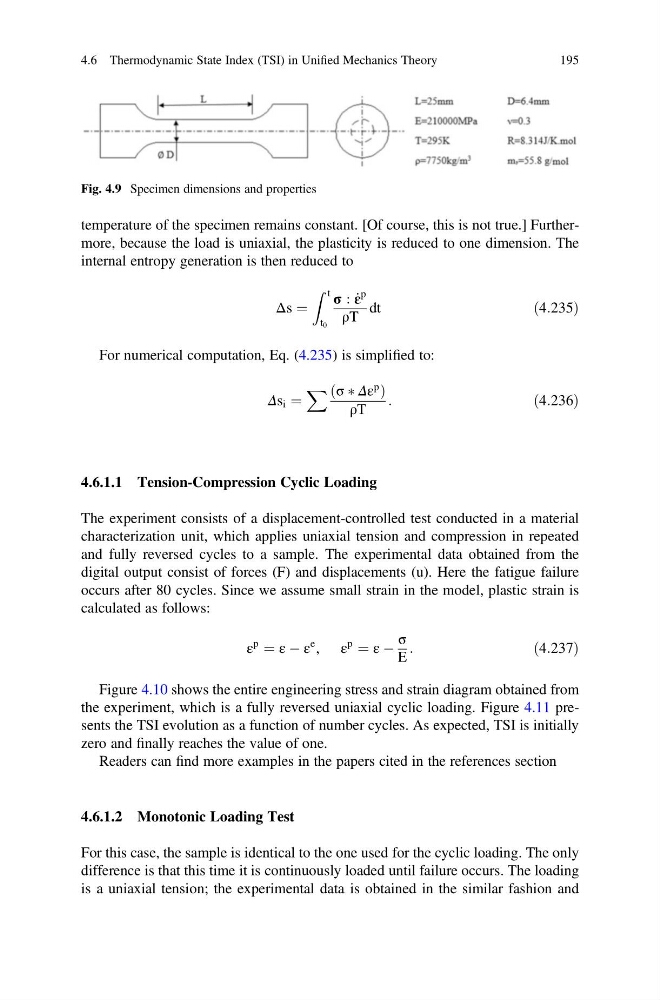
temperature of the specimen remains constant. [Of course, this is not true.] Furthermore, because the load is uniaxial, the plasticity is reduced to one dimension. The
internal entropy generation is then reduced to
Δs ¼
Z t
t 0
σ : _
ε
p
ρT
dt
ð4:235Þ
For numerical computation, Eq. (4.235) is simplified to:
Δs i ¼
X σ Ã Δε
p
ð
Þ
ρT
:
ð4:236Þ
4.6.1.1 Tension-Compression Cyclic Loading
The experiment consists of a displacement-controlled test conducted in a material
characterization unit, which applies uniaxial tension and compression in repeated
and fully reversed cycles to a sample. The experimental data obtained from the
digital output consist of forces (F) and displacements (u). Here the fatigue failure
occurs after 80 cycles. Since we assume small strain in the model, plastic strain is
calculated as follows:
ε
p
¼ ε À ε
e , ε
p
¼ ε À
σ
E
:
ð4:237Þ
Figure 4.10 shows the entire engineering stress and strain diagram obtained from
the experiment, which is a fully reversed uniaxial cyclic loading. Figure 4.11 presents the TSI evolution as a function of number cycles. As expected, TSI is initially
zero and finally reaches the value of one.
Readers can find more examples in the papers cited in the references section
4.6.1.2 Monotonic Loading Test
For this case, the sample is identical to the one used for the cyclic loading. The only
difference is that this time it is continuously loaded until failure occurs. The loading
is a uniaxial tension; the experimental data is obtained in the similar fashion and
Fig. 4.9 Specimen dimensions and properties
4.6 Thermodynamic State Index (TSI) in Unified Mechanics Theory
195
internal entropy generation is then reduced to
Δs ¼
Z t
t 0
σ : _
ε
p
ρT
dt
ð4:235Þ
For numerical computation, Eq. (4.235) is simplified to:
Δs i ¼
X σ Ã Δε
p
ð
Þ
ρT
:
ð4:236Þ
4.6.1.1 Tension-Compression Cyclic Loading
The experiment consists of a displacement-controlled test conducted in a material
characterization unit, which applies uniaxial tension and compression in repeated
and fully reversed cycles to a sample. The experimental data obtained from the
digital output consist of forces (F) and displacements (u). Here the fatigue failure
occurs after 80 cycles. Since we assume small strain in the model, plastic strain is
calculated as follows:
ε
p
¼ ε À ε
e , ε
p
¼ ε À
σ
E
:
ð4:237Þ
Figure 4.10 shows the entire engineering stress and strain diagram obtained from
the experiment, which is a fully reversed uniaxial cyclic loading. Figure 4.11 presents the TSI evolution as a function of number cycles. As expected, TSI is initially
zero and finally reaches the value of one.
Readers can find more examples in the papers cited in the references section
4.6.1.2 Monotonic Loading Test
For this case, the sample is identical to the one used for the cyclic loading. The only
difference is that this time it is continuously loaded until failure occurs. The loading
is a uniaxial tension; the experimental data is obtained in the similar fashion and
Fig. 4.9 Specimen dimensions and properties
4.6 Thermodynamic State Index (TSI) in Unified Mechanics Theory
195