

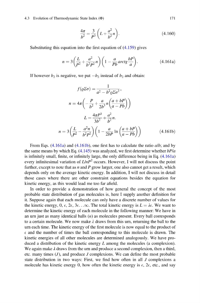
4π
b
2
¼
3
P
3
L þ
a
2
b
2
n
:
ð4:160Þ
Substituting this equation into the first equation of (4.159) gives
n ¼ 3
L
P
2
þ
a
2
b
2 P
2
n
1 À
a
Pb
arctg
bP
a
:
ð4:161aÞ
If however b 2 is negative, we put Àb 2 instead of b 2 and obtain:
f ϱΣσ
ð
Þ ¼
1
a 2 À b
2
ϱΣσ
2
,
n ¼ 4π À
P
b
2
þ
a
2b
3
n
a þ bP
a À Pb
L ¼
4πP
3
3b
2
þ
a
2
b
2
n:
n ¼ 3
L
P
2
À
a
2 n
b
2 P
2
1 À
a
2bP
ln
a þ bP
a À Pb
ð4:161bÞ
From Eqs. (4.161a) and (4.161b), one first has to calculate the ratio a/b; and by
the same means by which Eq. (4.145) was analyzed, we first determine whether bP/a
is infinitely small, finite, or infinitely large, the only difference being in Eq. (4.161a)
every infinitesimal variation of L/nP
2 occurs. However, I will not discuss the point
further, except to note that as n and P grow larger, one also cannot get a result, which
depends only on the average kinetic energy. In addition, I will not discuss in detail
those cases where there are other constraint equations besides the equation for
kinetic energy, as this would lead me too far afield.
In order to provide a demonstration of how general the concept of the most
probable state distribution of gas molecules is, here I supply another definition for
it. Suppose again that each molecule can only have a discrete number of values for
the kinetic energy, 0, E, 2E, 3E. . .1. The total kinetic energy is L ¼ λE. We want to
determine the kinetic energy of each molecule in the following manner: We have in
an urn just as many identical balls (n) as molecules present. Every ball corresponds
to a certain molecule. We now make λ draws from this urn, returning the ball to the
urn each time. The kinetic energy of the first molecule is now equal to the product of
E and the number of times the ball corresponding to this molecule is drawn. The
kinetic energies of all other molecules are determined analogously. We have produced a distribution of the kinetic energy L among the molecules (a complexion).
We again make λ draws from the urn and produce a second complexion, then a third,
etc. many times (J), and produce J complexions. We can define the most probable
state distribution in two ways: First, we find how often in all J complexions a
molecule has kinetic energy 0, how often the kinetic energy is E, 2E, etc., and say
4.3 Evolution of Thermodynamic State Index (Φ)
171
b
2
¼
3
P
3
L þ
a
2
b
2
n
:
ð4:160Þ
Substituting this equation into the first equation of (4.159) gives
n ¼ 3
L
P
2
þ
a
2
b
2 P
2
n
1 À
a
Pb
arctg
bP
a
:
ð4:161aÞ
If however b 2 is negative, we put Àb 2 instead of b 2 and obtain:
f ϱΣσ
ð
Þ ¼
1
a 2 À b
2
ϱΣσ
2
,
n ¼ 4π À
P
b
2
þ
a
2b
3
n
a þ bP
a À Pb
L ¼
4πP
3
3b
2
þ
a
2
b
2
n:
n ¼ 3
L
P
2
À
a
2 n
b
2 P
2
1 À
a
2bP
ln
a þ bP
a À Pb
ð4:161bÞ
From Eqs. (4.161a) and (4.161b), one first has to calculate the ratio a/b; and by
the same means by which Eq. (4.145) was analyzed, we first determine whether bP/a
is infinitely small, finite, or infinitely large, the only difference being in Eq. (4.161a)
every infinitesimal variation of L/nP
2 occurs. However, I will not discuss the point
further, except to note that as n and P grow larger, one also cannot get a result, which
depends only on the average kinetic energy. In addition, I will not discuss in detail
those cases where there are other constraint equations besides the equation for
kinetic energy, as this would lead me too far afield.
In order to provide a demonstration of how general the concept of the most
probable state distribution of gas molecules is, here I supply another definition for
it. Suppose again that each molecule can only have a discrete number of values for
the kinetic energy, 0, E, 2E, 3E. . .1. The total kinetic energy is L ¼ λE. We want to
determine the kinetic energy of each molecule in the following manner: We have in
an urn just as many identical balls (n) as molecules present. Every ball corresponds
to a certain molecule. We now make λ draws from this urn, returning the ball to the
urn each time. The kinetic energy of the first molecule is now equal to the product of
E and the number of times the ball corresponding to this molecule is drawn. The
kinetic energies of all other molecules are determined analogously. We have produced a distribution of the kinetic energy L among the molecules (a complexion).
We again make λ draws from the urn and produce a second complexion, then a third,
etc. many times (J), and produce J complexions. We can define the most probable
state distribution in two ways: First, we find how often in all J complexions a
molecule has kinetic energy 0, how often the kinetic energy is E, 2E, etc., and say
4.3 Evolution of Thermodynamic State Index (Φ)
171