

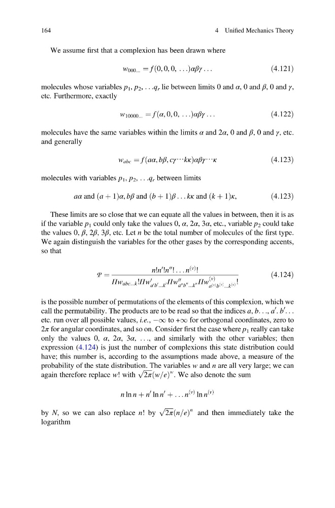
We assume first that a complexion has been drawn where
w 000... ¼ f 0, 0, 0, . . .
ð
Þ αβγ . . .
ð4:121Þ
molecules whose variables p 1 , p 2 , . . .q r lie between limits 0 and α, 0 and β, 0 and γ,
etc. Furthermore, exactly
w 10000... ¼ f α, 0, 0, . . .
ð
Þ αβγ . . .
ð4:122Þ
molecules have the same variables within the limits α and 2α, 0 and β, 0 and γ, etc.
and generally
w abc ¼ f aα, bβ, cγ⋯kκ
ð
Þ αβγ⋯κ
ð4:123Þ
molecules with variables p 1 , p 2 , . . .q r between limits
aα and a þ 1
ð
Þα, bβ and b þ 1
ð
Þβ . . . kκ and k þ 1
ð
Þκ,
ð4:123Þ
These limits are so close that we can equate all the values in between, then it is as
if the variable p 1 could only take the values 0, α, 2α, 3α, etc., variable p 2 could take
the values 0, β, 2β, 3β, etc. Let n be the total number of molecules of the first type.
We again distinguish the variables for the other gases by the corresponding accents,
so that
P ¼
n!n
0
!n
00
! . . . n
v
ð Þ
!
Πw abc...k !Πw 0
a 0 b
0 ...k
0 Πw 00
a 00 b
00 ...k
00 Πw
v
ð Þ
a v
ð Þ b
v
ð Þ ...k
v
ð Þ !
ð4:124Þ
is the possible number of permutations of the elements of this complexion, which we
call the permutability. The products are to be read so that the indices a, b. . ., a
0 . b
0
. . .
etc. run over all possible values, i.e., À1 to +1 for orthogonal coordinates, zero to
2π for angular coordinates, and so on. Consider first the case where p 1 really can take
only the values 0, α, 2α, 3α, . . ., and similarly with the other variables; then
expression (4.124) is just the number of complexions this state distribution could
have; this number is, according to the assumptions made above, a measure of the
probability of the state distribution. The variables w and n are all very large; we can
again therefore replace w! with
ffiffiffiffiffi
2π
p
w=e
ð
Þ
w . We also denote the sum
n ln n þ n
0 ln n
0
þ . . . n
v
ð Þ ln n
v
ð Þ
by N, so we can also replace n! by
ffiffiffiffiffi
2π
p
n=e
ð Þ
n and then immediately take the
logarithm
164
4 Unified Mechanics Theory
w 000... ¼ f 0, 0, 0, . . .
ð
Þ αβγ . . .
ð4:121Þ
molecules whose variables p 1 , p 2 , . . .q r lie between limits 0 and α, 0 and β, 0 and γ,
etc. Furthermore, exactly
w 10000... ¼ f α, 0, 0, . . .
ð
Þ αβγ . . .
ð4:122Þ
molecules have the same variables within the limits α and 2α, 0 and β, 0 and γ, etc.
and generally
w abc ¼ f aα, bβ, cγ⋯kκ
ð
Þ αβγ⋯κ
ð4:123Þ
molecules with variables p 1 , p 2 , . . .q r between limits
aα and a þ 1
ð
Þα, bβ and b þ 1
ð
Þβ . . . kκ and k þ 1
ð
Þκ,
ð4:123Þ
These limits are so close that we can equate all the values in between, then it is as
if the variable p 1 could only take the values 0, α, 2α, 3α, etc., variable p 2 could take
the values 0, β, 2β, 3β, etc. Let n be the total number of molecules of the first type.
We again distinguish the variables for the other gases by the corresponding accents,
so that
P ¼
n!n
0
!n
00
! . . . n
v
ð Þ
!
Πw abc...k !Πw 0
a 0 b
0 ...k
0 Πw 00
a 00 b
00 ...k
00 Πw
v
ð Þ
a v
ð Þ b
v
ð Þ ...k
v
ð Þ !
ð4:124Þ
is the possible number of permutations of the elements of this complexion, which we
call the permutability. The products are to be read so that the indices a, b. . ., a
0 . b
0
. . .
etc. run over all possible values, i.e., À1 to +1 for orthogonal coordinates, zero to
2π for angular coordinates, and so on. Consider first the case where p 1 really can take
only the values 0, α, 2α, 3α, . . ., and similarly with the other variables; then
expression (4.124) is just the number of complexions this state distribution could
have; this number is, according to the assumptions made above, a measure of the
probability of the state distribution. The variables w and n are all very large; we can
again therefore replace w! with
ffiffiffiffiffi
2π
p
w=e
ð
Þ
w . We also denote the sum
n ln n þ n
0 ln n
0
þ . . . n
v
ð Þ ln n
v
ð Þ
by N, so we can also replace n! by
ffiffiffiffiffi
2π
p
n=e
ð Þ
n and then immediately take the
logarithm
164
4 Unified Mechanics Theory