

M ¼ E f 0
ð Þ ln f 0
ð Þ þ f E
ð Þ ln f E
ð Þ þ f 2E
ð Þln f 2E
ð Þ þ . . .
½
þ E ln E f 0
ð Þ þ f E
ð Þ þ f 2E
ð Þ þ . . .
½
À n
ð4:87Þ
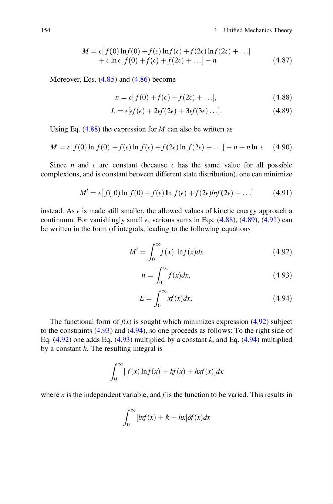
Moreover, Eqs. (4.85) and (4.86) become
n ¼ E f 0
ð Þ þ f E
ð Þ þ f 2E
ð Þ þ . . .
½
,
ð4:88Þ
L ¼ E Ef E
ð Þ þ 2Ef 2E
ð Þ þ 3Ef 3E
ð Þ. . .
½
:
ð4:89Þ
Using Eq. (4.88) the expression for M can also be written as
M ¼ E f 0
ð Þ ln f 0
ð Þ þ f E
ð Þ ln f E
ð Þ þ f 2E
ð Þln f 2E
ð Þ þ . . .
½
À n þ n ln E ð4:90Þ
Since n and E are constant (because E has the same value for all possible
complexions, and is constant between different state distribution), one can minimize
M
0
¼ E f 0
ð Þln f 0
ð Þ þ f E
ð Þ ln f E
ð Þ þ f 2E
ð Þlnf 2E
ð Þ þ . . .
½
ð 4:91Þ
instead. As E is made still smaller, the allowed values of kinetic energy approach a
continuum. For vanishingly small E, various sums in Eqs. (4.88), (4.89), (4.91) can
be written in the form of integrals, leading to the following equations
M
0
¼
Z 1
0
f x
ð Þ ln f x
ð Þdx
ð4:92Þ
n ¼
Z 1
0
f x
ð Þdx,
ð4:93Þ
L ¼
Z 1
0
xf x
ð Þdx,
ð4:94Þ
The functional form of f(x) is sought which minimizes expression (4.92) subject
to the constraints (4.93) and (4.94), so one proceeds as follows: To the right side of
Eq. (4.92) one adds Eq. (4.93) multiplied by a constant k, and Eq. (4.94) multiplied
by a constant h. The resulting integral is
Z 1
0
f x
ð Þ ln f x
ð Þ þ kf x
ð Þ þ hxf x
ð Þ
½
dx
where x is the independent variable, and f is the function to be varied. This results in
Z 1
0
lnf x
ð Þ þ k þ hx
½
δf x
ð Þdx
154
4 Unified Mechanics Theory
ð Þ ln f 0
ð Þ þ f E
ð Þ ln f E
ð Þ þ f 2E
ð Þln f 2E
ð Þ þ . . .
½
þ E ln E f 0
ð Þ þ f E
ð Þ þ f 2E
ð Þ þ . . .
½
À n
ð4:87Þ
Moreover, Eqs. (4.85) and (4.86) become
n ¼ E f 0
ð Þ þ f E
ð Þ þ f 2E
ð Þ þ . . .
½
,
ð4:88Þ
L ¼ E Ef E
ð Þ þ 2Ef 2E
ð Þ þ 3Ef 3E
ð Þ. . .
½
:
ð4:89Þ
Using Eq. (4.88) the expression for M can also be written as
M ¼ E f 0
ð Þ ln f 0
ð Þ þ f E
ð Þ ln f E
ð Þ þ f 2E
ð Þln f 2E
ð Þ þ . . .
½
À n þ n ln E ð4:90Þ
Since n and E are constant (because E has the same value for all possible
complexions, and is constant between different state distribution), one can minimize
M
0
¼ E f 0
ð Þln f 0
ð Þ þ f E
ð Þ ln f E
ð Þ þ f 2E
ð Þlnf 2E
ð Þ þ . . .
½
ð 4:91Þ
instead. As E is made still smaller, the allowed values of kinetic energy approach a
continuum. For vanishingly small E, various sums in Eqs. (4.88), (4.89), (4.91) can
be written in the form of integrals, leading to the following equations
M
0
¼
Z 1
0
f x
ð Þ ln f x
ð Þdx
ð4:92Þ
n ¼
Z 1
0
f x
ð Þdx,
ð4:93Þ
L ¼
Z 1
0
xf x
ð Þdx,
ð4:94Þ
The functional form of f(x) is sought which minimizes expression (4.92) subject
to the constraints (4.93) and (4.94), so one proceeds as follows: To the right side of
Eq. (4.92) one adds Eq. (4.93) multiplied by a constant k, and Eq. (4.94) multiplied
by a constant h. The resulting integral is
Z 1
0
f x
ð Þ ln f x
ð Þ þ kf x
ð Þ þ hxf x
ð Þ
½
dx
where x is the independent variable, and f is the function to be varied. This results in
Z 1
0
lnf x
ð Þ þ k þ hx
½
δf x
ð Þdx
154
4 Unified Mechanics Theory