

480
12 Nonlinear Processes in Optical Fibers
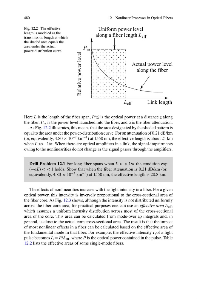
Fig. 12.2 The effective
length is modeled as the
transmission length at which
the shaded area equals the
area under the actual
power-distribution curve
Here L is the length of the fiber span, P(z) is the optical power at a distance z along
the fiber, P in is the power level launched into the fiber, and α is the fiber attenuation.
As Fig. 12.2 illustrates, this means that the area designated by the shaded pattern is
equal to the area under the power-distribution curve. For an attenuation of 0.21 dB/km
(or, equivalently, 4.80 × 10
−2 km
−1 ) at 1550 nm, the effective length is about 21 km
when L >> 1/α. When there are optical amplifiers in a link, the signal-impairments
owing to the nonlinearities do not change as the signal passes through the amplifiers.
Drill Problem 12.1 For long fiber spans when L > > 1/α the condition exp
(−αL) < < 1 holds. Show that when the fiber attenuation is 0.21 dB/km (or,
equivalently, 4.80 × 10
−2 km
−1 ) at 1550 nm, the effective length is 20.8 km.
The effects of nonlinearities increase with the light intensity in a fiber. For a given
optical power, this intensity is inversely proportional to the cross-sectional area of
the fiber core. As Fig. 12.3 shows, although the intensity is not distributed uniformly
across the fiber-core area, for practical purposes one can use an effective area A eff ,
which assumes a uniform intensity distribution across most of the cross-sectional
area of the core. This area can be calculated from mode-overlap integrals and, in
general, is close to the actual core cross-sectional area. The result is that the impact
of most nonlinear effects in a fiber can be calculated based on the effective area of
the fundamental mode in that fiber. For example, the effective intensity I e of a light
pulse becomes I e = P/A eff , where P is the optical power contained in the pulse. Table
12.2 lists the effective areas of some single-mode fibers.
12 Nonlinear Processes in Optical Fibers
Fig. 12.2 The effective
length is modeled as the
transmission length at which
the shaded area equals the
area under the actual
power-distribution curve
Here L is the length of the fiber span, P(z) is the optical power at a distance z along
the fiber, P in is the power level launched into the fiber, and α is the fiber attenuation.
As Fig. 12.2 illustrates, this means that the area designated by the shaded pattern is
equal to the area under the power-distribution curve. For an attenuation of 0.21 dB/km
(or, equivalently, 4.80 × 10
−2 km
−1 ) at 1550 nm, the effective length is about 21 km
when L >> 1/α. When there are optical amplifiers in a link, the signal-impairments
owing to the nonlinearities do not change as the signal passes through the amplifiers.
Drill Problem 12.1 For long fiber spans when L > > 1/α the condition exp
(−αL) < < 1 holds. Show that when the fiber attenuation is 0.21 dB/km (or,
equivalently, 4.80 × 10
−2 km
−1 ) at 1550 nm, the effective length is 20.8 km.
The effects of nonlinearities increase with the light intensity in a fiber. For a given
optical power, this intensity is inversely proportional to the cross-sectional area of
the fiber core. As Fig. 12.3 shows, although the intensity is not distributed uniformly
across the fiber-core area, for practical purposes one can use an effective area A eff ,
which assumes a uniform intensity distribution across most of the cross-sectional
area of the core. This area can be calculated from mode-overlap integrals and, in
general, is close to the actual core cross-sectional area. The result is that the impact
of most nonlinear effects in a fiber can be calculated based on the effective area of
the fundamental mode in that fiber. For example, the effective intensity I e of a light
pulse becomes I e = P/A eff , where P is the optical power contained in the pulse. Table
12.2 lists the effective areas of some single-mode fibers.