

5.2 Coupling Improvement with Lensing Schemes
221
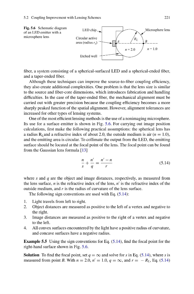
Fig. 5.6 Schematic diagram
of an LED emitter with a
microsphere lens
fiber, a system consisting of a spherical-surfaced LED and a spherical-ended fiber,
and a taper-ended fiber.
Although these techniques can improve the source-to-fiber coupling efficiency,
they also create additional complexities. One problem is that the lens size is similar
to the source and fiber-core dimensions, which introduces fabrication and handling
difficulties. In the case of the taper-ended fiber, the mechanical alignment must be
carried out with greater precision because the coupling efficiency becomes a more
sharply peaked function of the spatial alignment. However, alignment tolerances are
increased for other types of lensing systems.
One of the most efficient lensing methods is the use of a nonimaging microsphere.
Its use for a surface emitter is shown in Fig. 5.6. For carrying out image position
calculations, first make the following practical assumptions: the spherical lens has
a radius R L and a refractive index of about 2.0, the outside medium is air (n = 1.0),
and the emitting area is circular. To collimate the output from the LED, the emitting
surface should be located at the focal point of the lens. The focal point can be found
from the Gaussian lens formula [13]
n
s
+
n
q
=
n
− n
r
(5.14)
where s and q are the object and image distances, respectively, as measured from
the lens surface, n is the refractive index of the lens, n
is the refractive index of the
outside medium, and r is the radius of curvature of the lens surface.
The following sign conventions are used with Eq. (5.14):
1. Light travels from left to right.
2. Object distances are measured as positive to the left of a vertex and negative to
the right.
3. Image distances are measured as positive to the right of a vertex and negative
to the left.
4. All convex surfaces encountered by the light have a positive radius of curvature,
and concave surfaces have a negative radius.
Example 5.5 Using the sign conventions for Eq. (5.14), find the focal point for the
right-hand surface shown in Fig. 5.6.
Solution To find the focal point, set q = ∞ and solve for s in Eq. (5.14), where s is
measured from point B. With n = 2.0, n
= 1.0, q = ∞, and r = − R L , Eq. (5.14)
221
Fig. 5.6 Schematic diagram
of an LED emitter with a
microsphere lens
fiber, a system consisting of a spherical-surfaced LED and a spherical-ended fiber,
and a taper-ended fiber.
Although these techniques can improve the source-to-fiber coupling efficiency,
they also create additional complexities. One problem is that the lens size is similar
to the source and fiber-core dimensions, which introduces fabrication and handling
difficulties. In the case of the taper-ended fiber, the mechanical alignment must be
carried out with greater precision because the coupling efficiency becomes a more
sharply peaked function of the spatial alignment. However, alignment tolerances are
increased for other types of lensing systems.
One of the most efficient lensing methods is the use of a nonimaging microsphere.
Its use for a surface emitter is shown in Fig. 5.6. For carrying out image position
calculations, first make the following practical assumptions: the spherical lens has
a radius R L and a refractive index of about 2.0, the outside medium is air (n = 1.0),
and the emitting area is circular. To collimate the output from the LED, the emitting
surface should be located at the focal point of the lens. The focal point can be found
from the Gaussian lens formula [13]
n
s
+
n
q
=
n
− n
r
(5.14)
where s and q are the object and image distances, respectively, as measured from
the lens surface, n is the refractive index of the lens, n
is the refractive index of the
outside medium, and r is the radius of curvature of the lens surface.
The following sign conventions are used with Eq. (5.14):
1. Light travels from left to right.
2. Object distances are measured as positive to the left of a vertex and negative to
the right.
3. Image distances are measured as positive to the right of a vertex and negative
to the left.
4. All convex surfaces encountered by the light have a positive radius of curvature,
and concave surfaces have a negative radius.
Example 5.5 Using the sign conventions for Eq. (5.14), find the focal point for the
right-hand surface shown in Fig. 5.6.
Solution To find the focal point, set q = ∞ and solve for s in Eq. (5.14), where s is
measured from point B. With n = 2.0, n
= 1.0, q = ∞, and r = − R L , Eq. (5.14)