

5.1 Source-to-Fiber Power Coupling
213
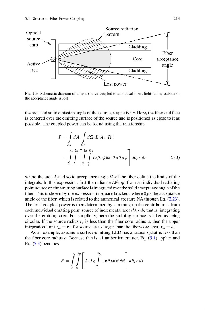
Fig. 5.3 Schematic diagram of a light source coupled to an optical fiber; light falling outside of
the acceptance angle is lost
the area and solid emission angle of the source, respectively. Here, the fiber end face
is centered over the emitting surface of the source and is positioned as close to it as
possible. The coupled power can be found using the relationship
P =
A f
d A s
f
d s L(A s , , s )
=
r m
0
2π
0
⎡
⎣
2π
0
A
0
L(θ, φ)sinθ dθ dφ
⎤
⎦ dθ s r dr
(5.3)
where the area A f and solid acceptance angle f of the fiber define the limits of the
integrals. In this expression, first the radiance L(θ, ϕ) from an individual radiating
point source on the emitting surface is integrated over the solid acceptance angle of the
fiber. This is shown by the expression in square brackets, where θ A is the acceptance
angle of the fiber, which is related to the numerical aperture NA through Eq. (2.23).
The total coupled power is then determined by summing up the contributions from
each individual emitting point source of incremental area dθ s r dr, that is, integrating
over the emitting area. For simplicity, here the emitting surface is taken as being
circular. If the source radius r s is less than the fiber core radius a, then the upper
integration limit r m = r s ; for source areas larger than the fiber-core area, r m = a.
As an example, assume a surface-emitting LED has a radius r s that is less than
the fiber core radius a. Because this is a Lambertian emitter, Eq. (5.1) applies and
Eq. (5.3) becomes
P =
r s
0
2π
0
⎡
⎣ 2π L 0
A
0
cosθ sinθ dθ
⎤
⎦ dθ s r dr
213
Fig. 5.3 Schematic diagram of a light source coupled to an optical fiber; light falling outside of
the acceptance angle is lost
the area and solid emission angle of the source, respectively. Here, the fiber end face
is centered over the emitting surface of the source and is positioned as close to it as
possible. The coupled power can be found using the relationship
P =
A f
d A s
f
d s L(A s , , s )
=
r m
0
2π
0
⎡
⎣
2π
0
A
0
L(θ, φ)sinθ dθ dφ
⎤
⎦ dθ s r dr
(5.3)
where the area A f and solid acceptance angle f of the fiber define the limits of the
integrals. In this expression, first the radiance L(θ, ϕ) from an individual radiating
point source on the emitting surface is integrated over the solid acceptance angle of the
fiber. This is shown by the expression in square brackets, where θ A is the acceptance
angle of the fiber, which is related to the numerical aperture NA through Eq. (2.23).
The total coupled power is then determined by summing up the contributions from
each individual emitting point source of incremental area dθ s r dr, that is, integrating
over the emitting area. For simplicity, here the emitting surface is taken as being
circular. If the source radius r s is less than the fiber core radius a, then the upper
integration limit r m = r s ; for source areas larger than the fiber-core area, r m = a.
As an example, assume a surface-emitting LED has a radius r s that is less than
the fiber core radius a. Because this is a Lambertian emitter, Eq. (5.1) applies and
Eq. (5.3) becomes
P =
r s
0
2π
0
⎡
⎣ 2π L 0
A
0
cosθ sinθ dθ
⎤
⎦ dθ s r dr