

yields
ln
A
½
A
½ 0
= −kt
(3.21)
Taking exponentials of both sides gives
A
½
A
½ 0
= e
−kt
(3.22)
which can be rearranged to the final form
A
½ = A
½ 0 e
−kt
(3.23)
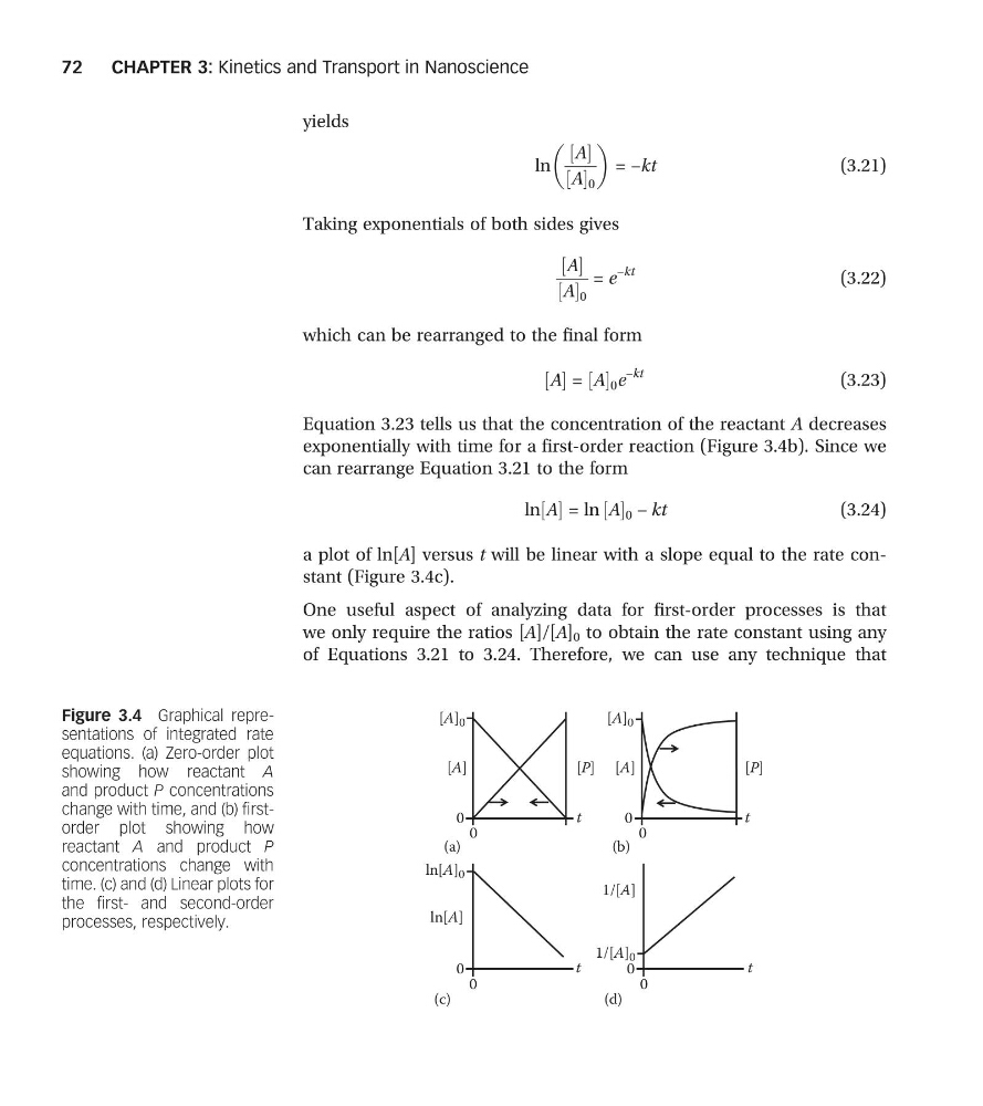
Equation 3.23 tells us that the concentration of the reactant A decreases
exponentially with time for a first-order reaction (Figure 3.4b). Since we
can rearrange Equation 3.21 to the form
ln A
½ = ln A
½ 0 − kt
(3.24)
a plot of ln[A] versus t will be linear with a slope equal to the rate constant (Figure 3.4c).
One useful aspect of analyzing data for first-order processes is that
we only require the ratios [A]/[A] 0 to obtain the rate constant using any
of Equations 3.21 to 3.24. Therefore, we can use any technique that
[A]
[ A]
t
t
t
[A] 0
[A] 0
ln[A]
ln[A] 0
1/[A]
1/[A] 0
[P]
t
[P]
0
0
0
0
0
0
0
0
(a)
(b)
(c)
(d)
Figure 3.4 Graphical representations of integrated rate
equations. (a) Zero-order plot
showing how reactant A
and product P concentrations
change with time, and (b) firstorder plot showing how
reactant A and product P
concentrations change with
time. (c) and (d) Linear plots for
the first- and second-order
processes, respectively.
CHAPTER 3: Kinetics and Transport in Nanoscience
72
ln
A
½
A
½ 0
= −kt
(3.21)
Taking exponentials of both sides gives
A
½
A
½ 0
= e
−kt
(3.22)
which can be rearranged to the final form
A
½ = A
½ 0 e
−kt
(3.23)
Equation 3.23 tells us that the concentration of the reactant A decreases
exponentially with time for a first-order reaction (Figure 3.4b). Since we
can rearrange Equation 3.21 to the form
ln A
½ = ln A
½ 0 − kt
(3.24)
a plot of ln[A] versus t will be linear with a slope equal to the rate constant (Figure 3.4c).
One useful aspect of analyzing data for first-order processes is that
we only require the ratios [A]/[A] 0 to obtain the rate constant using any
of Equations 3.21 to 3.24. Therefore, we can use any technique that
[A]
[ A]
t
t
t
[A] 0
[A] 0
ln[A]
ln[A] 0
1/[A]
1/[A] 0
[P]
t
[P]
0
0
0
0
0
0
0
0
(a)
(b)
(c)
(d)
Figure 3.4 Graphical representations of integrated rate
equations. (a) Zero-order plot
showing how reactant A
and product P concentrations
change with time, and (b) firstorder plot showing how
reactant A and product P
concentrations change with
time. (c) and (d) Linear plots for
the first- and second-order
processes, respectively.
CHAPTER 3: Kinetics and Transport in Nanoscience
72