

3.1.4 Integrated rate laws
The explicit relationship between the concentration of a reactant and time
can be obtained by integrating rate laws with respect to time. These
relationships, known as integrated rate laws, can be used to determine the
concentration of a reactant at any given time or to determine the rate
constant from a series of concentrations at different times. As a concrete
example, let’s consider the following first-order reaction:
A⟶
k products
(3.17)
Equation 3.18 describes the rate law corresponding to this first-order
process:
−
d A
½
dt
= k A
½
(3.18)
This equation can be rearranged such that concentration terms are on the
left-hand side and time is on the right-hand side (Equation 3.19):
1
A
½
d A
½ = −kdt
(3.19)
Integrating the above equation from the initial concentration [A] 0 at t = 0
to some final concentration [A] at time t, or mathematically,
ð A
½
A
½ 0
1
A
½
d A
½ = −k
ð t
0
dt
(3.20)
[A]
Time
[A] 0
[B] 0
0
0
[P]
(a)
(b)
[B]
[B] eq
[A] eq
[P] eq
[B] eq
[A] eq
[P] eq
[A]
[P]
[B]
Concentration
[A] 0
[B] 0
0
Concentration
t eq
Time
0
t eq
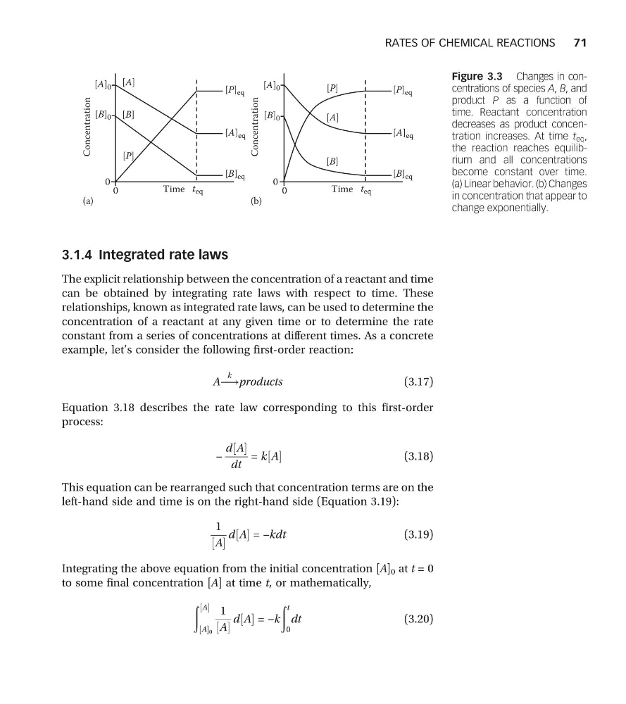
Figure 3.3 Changes in concentrations of species A, B, and
product P as a function of
time. Reactant concentration
decreases as product concentration increases. At time t eq ,
the reaction reaches equilibrium and all concentrations
become constant over time.
(a) Linear behavior. (b) Changes
in concentration that appear to
change exponentially.
RATES OF CHEMICAL REACTIONS
71
The explicit relationship between the concentration of a reactant and time
can be obtained by integrating rate laws with respect to time. These
relationships, known as integrated rate laws, can be used to determine the
concentration of a reactant at any given time or to determine the rate
constant from a series of concentrations at different times. As a concrete
example, let’s consider the following first-order reaction:
A⟶
k products
(3.17)
Equation 3.18 describes the rate law corresponding to this first-order
process:
−
d A
½
dt
= k A
½
(3.18)
This equation can be rearranged such that concentration terms are on the
left-hand side and time is on the right-hand side (Equation 3.19):
1
A
½
d A
½ = −kdt
(3.19)
Integrating the above equation from the initial concentration [A] 0 at t = 0
to some final concentration [A] at time t, or mathematically,
ð A
½
A
½ 0
1
A
½
d A
½ = −k
ð t
0
dt
(3.20)
[A]
Time
[A] 0
[B] 0
0
0
[P]
(a)
(b)
[B]
[B] eq
[A] eq
[P] eq
[B] eq
[A] eq
[P] eq
[A]
[P]
[B]
Concentration
[A] 0
[B] 0
0
Concentration
t eq
Time
0
t eq
Figure 3.3 Changes in concentrations of species A, B, and
product P as a function of
time. Reactant concentration
decreases as product concentration increases. At time t eq ,
the reaction reaches equilibrium and all concentrations
become constant over time.
(a) Linear behavior. (b) Changes
in concentration that appear to
change exponentially.
RATES OF CHEMICAL REACTIONS
71