

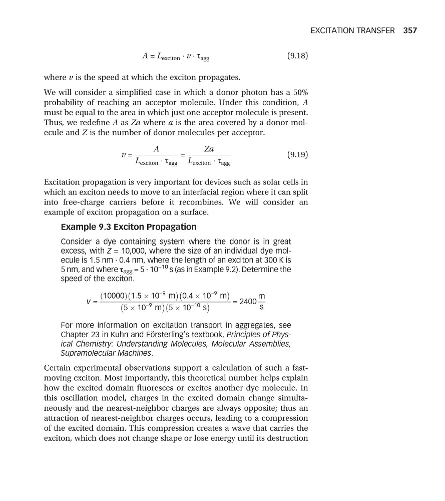
A = L exciton Á v Á t agg
(9.18)
where v is the speed at which the exciton propagates.
We will consider a simplified case in which a donor photon has a 50%
probability of reaching an acceptor molecule. Under this condition, A
must be equal to the area in which just one acceptor molecule is present.
Thus, we redefine A as Za where a is the area covered by a donor molecule and Z is the number of donor molecules per acceptor.
v =
A
L exciton Á t agg
=
Za
L exciton Á t agg
(9.19)
Excitation propagation is very important for devices such as solar cells in
which an exciton needs to move to an interfacial region where it can split
into free-charge carriers before it recombines. We will consider an
example of exciton propagation on a surface.
Example 9.3 Exciton Propagation
Consider a dye containing system where the donor is in great
excess, with Z = 10,000, where the size of an individual dye molecule is 1.5 nm · 0.4 nm, where the length of an exciton at 300 K is
5 nm, and where τ agg = 5 · 10
−10 s (as in Example 9.2). Determine the
speed of the exciton.
v =
10000
ð
Þ 1:5 Â 10
−9 m
À
Á
0:4 Â 10
−9 m
À
Á
5 Â 10
−9 m
À
Á
5 Â 10
−10 s
À
Á
= 2400
m
s
For more information on excitation transport in aggregates, see
Chapter 23 in Kuhn and Försterling’s textbook, Principles of Physical Chemistry: Understanding Molecules, Molecular Assemblies,
Supramolecular Machines.
Certain experimental observations support a calculation of such a fastmoving exciton. Most importantly, this theoretical number helps explain
how the excited domain fluoresces or excites another dye molecule. In
this oscillation model, charges in the excited domain change simultaneously and the nearest-neighbor charges are always opposite; thus an
attraction of nearest-neighbor charges occurs, leading to a compression
of the excited domain. This compression creates a wave that carries the
exciton, which does not change shape or lose energy until its destruction
EXCITATION TRANSFER 357
(9.18)
where v is the speed at which the exciton propagates.
We will consider a simplified case in which a donor photon has a 50%
probability of reaching an acceptor molecule. Under this condition, A
must be equal to the area in which just one acceptor molecule is present.
Thus, we redefine A as Za where a is the area covered by a donor molecule and Z is the number of donor molecules per acceptor.
v =
A
L exciton Á t agg
=
Za
L exciton Á t agg
(9.19)
Excitation propagation is very important for devices such as solar cells in
which an exciton needs to move to an interfacial region where it can split
into free-charge carriers before it recombines. We will consider an
example of exciton propagation on a surface.
Example 9.3 Exciton Propagation
Consider a dye containing system where the donor is in great
excess, with Z = 10,000, where the size of an individual dye molecule is 1.5 nm · 0.4 nm, where the length of an exciton at 300 K is
5 nm, and where τ agg = 5 · 10
−10 s (as in Example 9.2). Determine the
speed of the exciton.
v =
10000
ð
Þ 1:5 Â 10
−9 m
À
Á
0:4 Â 10
−9 m
À
Á
5 Â 10
−9 m
À
Á
5 Â 10
−10 s
À
Á
= 2400
m
s
For more information on excitation transport in aggregates, see
Chapter 23 in Kuhn and Försterling’s textbook, Principles of Physical Chemistry: Understanding Molecules, Molecular Assemblies,
Supramolecular Machines.
Certain experimental observations support a calculation of such a fastmoving exciton. Most importantly, this theoretical number helps explain
how the excited domain fluoresces or excites another dye molecule. In
this oscillation model, charges in the excited domain change simultaneously and the nearest-neighbor charges are always opposite; thus an
attraction of nearest-neighbor charges occurs, leading to a compression
of the excited domain. This compression creates a wave that carries the
exciton, which does not change shape or lose energy until its destruction
EXCITATION TRANSFER 357