

symmetry of the system, it may be more convenient to use Cartesian (e.g.,
particle on a sheet), spherical (e.g., hydrogen atom), or radial (e.g., particle on a ring) coordinates. We must then define the boundaries of
the system and define our Hamiltonian operator based on the model.
Finally, we must determine the wavefunctions that fit the constraints of
the Hamiltonian operator and the boundary conditions.
Once a wavefunction has been found, the final step is to interpret the
wavefunction to provide insight into how our system behaves. We will
begin by considering the simple case of an electron confined to a onedimensional region (a line). We will provide a descriptive rationale for
what the wavefunction in this model should look like. Usually, determining wavefunctions requires a more complex mathematical treatment
of the model, but this is beyond the scope of this book. Instead, the general
form will be provided and this, with the appropriate Hamiltonian operator,
will be used in the Schrödinger equation to solve for the eigenvalues, the
set of quantized energy states of the system. The mathematical form of
the wavefunction will also allow us to describe the position of the electron
in terms of probability. This one-dimensional model will then be generalized to describe two (square) and three-dimensional (cube) regions by
the simple extension of the one-dimensional wavefunction.
4.3 CONFINEMENT OF ELECTRONS IN BOXES
4.3.1 The one-dimensional model
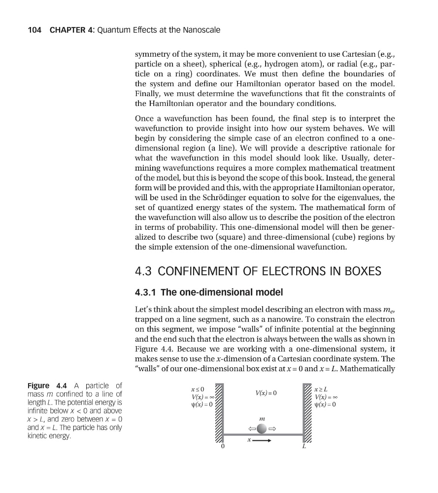
Let’s think about the simplest model describing an electron with mass m e ,
trapped on a line segment, such as a nanowire. To constrain the electron
on this segment, we impose “walls” of infinite potential at the beginning
and the end such that the electron is always between the walls as shown in
Figure 4.4. Because we are working with a one-dimensional system, it
makes sense to use the x-dimension of a Cartesian coordinate system. The
“walls” of our one-dimensional box exist at x = 0 and x = L. Mathematically
x ≤ 0
V(x) = ∞
V(x) = 0
0
m
x
L
ψ(x) = 0
x ≥ L
V(x) = ∞
ψ(x) = 0
Figure 4.4 A particle of
mass m confined to a line of
length L. The potential energy is
infinite below x < 0 and above
x > L, and zero between x = 0
and x = L. The particle has only
kinetic energy.
CHAPTER 4: Quantum Effects at the Nanoscale
104
particle on a sheet), spherical (e.g., hydrogen atom), or radial (e.g., particle on a ring) coordinates. We must then define the boundaries of
the system and define our Hamiltonian operator based on the model.
Finally, we must determine the wavefunctions that fit the constraints of
the Hamiltonian operator and the boundary conditions.
Once a wavefunction has been found, the final step is to interpret the
wavefunction to provide insight into how our system behaves. We will
begin by considering the simple case of an electron confined to a onedimensional region (a line). We will provide a descriptive rationale for
what the wavefunction in this model should look like. Usually, determining wavefunctions requires a more complex mathematical treatment
of the model, but this is beyond the scope of this book. Instead, the general
form will be provided and this, with the appropriate Hamiltonian operator,
will be used in the Schrödinger equation to solve for the eigenvalues, the
set of quantized energy states of the system. The mathematical form of
the wavefunction will also allow us to describe the position of the electron
in terms of probability. This one-dimensional model will then be generalized to describe two (square) and three-dimensional (cube) regions by
the simple extension of the one-dimensional wavefunction.
4.3 CONFINEMENT OF ELECTRONS IN BOXES
4.3.1 The one-dimensional model
Let’s think about the simplest model describing an electron with mass m e ,
trapped on a line segment, such as a nanowire. To constrain the electron
on this segment, we impose “walls” of infinite potential at the beginning
and the end such that the electron is always between the walls as shown in
Figure 4.4. Because we are working with a one-dimensional system, it
makes sense to use the x-dimension of a Cartesian coordinate system. The
“walls” of our one-dimensional box exist at x = 0 and x = L. Mathematically
x ≤ 0
V(x) = ∞
V(x) = 0
0
m
x
L
ψ(x) = 0
x ≥ L
V(x) = ∞
ψ(x) = 0
Figure 4.4 A particle of
mass m confined to a line of
length L. The potential energy is
infinite below x < 0 and above
x > L, and zero between x = 0
and x = L. The particle has only
kinetic energy.
CHAPTER 4: Quantum Effects at the Nanoscale
104