

d I
½
dt
= 0
(3.34)
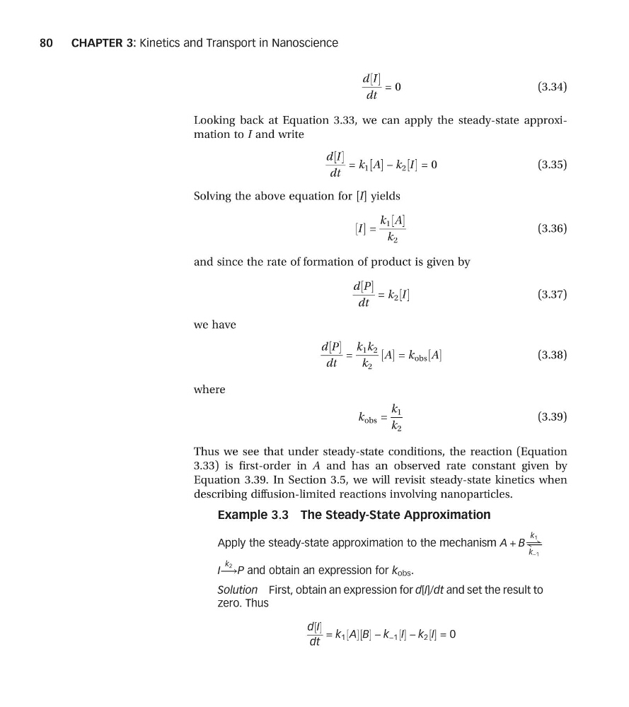
Looking back at Equation 3.33, we can apply the steady-state approximation to I and write
d I
½
dt
= k 1 A
½ − k 2 I
½ = 0
(3.35)
Solving the above equation for [I] yields
I
½ =
k 1 A
½
k 2
(3.36)
and since the rate of formation of product is given by
d P
½
dt
= k 2 I
½
(3.37)
we have
d P
½
dt
=
k 1 k 2
k 2
A
½ = k obs A
½
(3.38)
where
k obs =
k 1
k 2
(3.39)
Thus we see that under steady-state conditions, the reaction (Equation
3.33) is first-order in A and has an observed rate constant given by
Equation 3.39. In Section 3.5, we will revisit steady-state kinetics when
describing diffusion-limited reactions involving nanoparticles.
Example 3.3 The Steady-State Approximation
Apply the steady-state approximation to the mechanism A + B⇌
k 1
k −1
I⟶
k 2 P and obtain an expression for k obs .
Solution First, obtain an expression for d[I]/dt and set the result to
zero. Thus
d I
½
dt
= k 1 A
½ B
½ − k −1 I
½ − k 2 I
½ = 0
CHAPTER 3: Kinetics and Transport in Nanoscience
80
½
dt
= 0
(3.34)
Looking back at Equation 3.33, we can apply the steady-state approximation to I and write
d I
½
dt
= k 1 A
½ − k 2 I
½ = 0
(3.35)
Solving the above equation for [I] yields
I
½ =
k 1 A
½
k 2
(3.36)
and since the rate of formation of product is given by
d P
½
dt
= k 2 I
½
(3.37)
we have
d P
½
dt
=
k 1 k 2
k 2
A
½ = k obs A
½
(3.38)
where
k obs =
k 1
k 2
(3.39)
Thus we see that under steady-state conditions, the reaction (Equation
3.33) is first-order in A and has an observed rate constant given by
Equation 3.39. In Section 3.5, we will revisit steady-state kinetics when
describing diffusion-limited reactions involving nanoparticles.
Example 3.3 The Steady-State Approximation
Apply the steady-state approximation to the mechanism A + B⇌
k 1
k −1
I⟶
k 2 P and obtain an expression for k obs .
Solution First, obtain an expression for d[I]/dt and set the result to
zero. Thus
d I
½
dt
= k 1 A
½ B
½ − k −1 I
½ − k 2 I
½ = 0
CHAPTER 3: Kinetics and Transport in Nanoscience
80