

(in comparison with Austria, for example). Probably, the final size and the duration
of the epidemic in Germany have to be re-estimated taking into account possible
new waves of the epidemic, which can occur after the second T c .
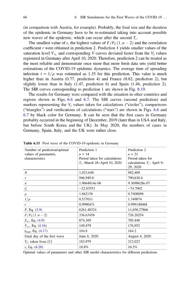
The smallest value of e, the highest values of F=F C ð1; n À 2Þ and the correlation
coefficient r were obtained in prediction 2. Prediction 1 yields smaller values of the
saturation level V 1 and corresponding V curves deviated faster from the V j values
registered in Germany after April 10, 2020. Therefore, prediction 2 can be treated as
the most reliable and demonstrate once more that more fresh data sets yield better
estimations of the COVID-19 epidemic dynamics. The average time of spreading
infection s ¼ 1=q was estimated as 1.35 for this prediction. This value is much
higher than in Austria (0.77, prediction 4) and France (0.82, prediction 2), but
slightly lower than in Italy (1.47, prediction 6) and Spain (1.46, prediction 2).
The SIR curves corresponding to prediction 1 are shown in Fig. 6.19.
The results for Germany were compared with the situation in other countries and
regions shown in Figs. 6.6 and 6.7. The SIR curves (second prediction) and
markers representing the V j values taken for calculations (“circles”), comparisons
(“triangles”) and verifications of calculations (“stars”) are shown in Figs. 6.6 and
6.7 by black color for Germany. It can be seen that the first cases in Germany
probably occurred in the beginning of December, 2019 (later than in USA and Italy,
but before South Korea and the UK). In May 2020, the numbers of cases in
Germany, Spain, Italy, and the UK were rather close.
Table 6.15 First wave of the COVID-19 epidemic in Germany
Number of prediction/optimal
values of parameters,
characteristics
Prediction 1
n = 14
Period taken for calculations
T c : March 28–April 10, 2020
Prediction 2
n = 21
Period taken for
calculations T c : April 9–
29, 2020
N
1,023,648
882,400
m
946,949.0
790,630.4
a
1.9664814e-06
9.3698628e-07
t
Ã
1
−22.83551
−74.7002
q
1.862158
0.7408098
1=q
0.537011
1.349874
r
0.9990431
0.999140468
F, Eq. (2.9)
6261.40324
11,038.27866
F=F C ð1; n À 2Þ
336.63458
726.20254
S 1 , Eq. (4.9)
874,169
705,448
V 1 , Eq. (4.16)
149,479
176,952
t final , Eq. (4.17)
104.8
164.2
Final day of the first wave
June 6, 2020
August 4, 2020
V f , taken from [1]
183,979
212,022
e, Eq. (4.20)
18.8%
16.5%
Optimal values of parameters and other SIR model characteristics for different predictions
66
6 SIR Simulations for the First Waves of the COVID-19 …
of the epidemic in Germany have to be re-estimated taking into account possible
new waves of the epidemic, which can occur after the second T c .
The smallest value of e, the highest values of F=F C ð1; n À 2Þ and the correlation
coefficient r were obtained in prediction 2. Prediction 1 yields smaller values of the
saturation level V 1 and corresponding V curves deviated faster from the V j values
registered in Germany after April 10, 2020. Therefore, prediction 2 can be treated as
the most reliable and demonstrate once more that more fresh data sets yield better
estimations of the COVID-19 epidemic dynamics. The average time of spreading
infection s ¼ 1=q was estimated as 1.35 for this prediction. This value is much
higher than in Austria (0.77, prediction 4) and France (0.82, prediction 2), but
slightly lower than in Italy (1.47, prediction 6) and Spain (1.46, prediction 2).
The SIR curves corresponding to prediction 1 are shown in Fig. 6.19.
The results for Germany were compared with the situation in other countries and
regions shown in Figs. 6.6 and 6.7. The SIR curves (second prediction) and
markers representing the V j values taken for calculations (“circles”), comparisons
(“triangles”) and verifications of calculations (“stars”) are shown in Figs. 6.6 and
6.7 by black color for Germany. It can be seen that the first cases in Germany
probably occurred in the beginning of December, 2019 (later than in USA and Italy,
but before South Korea and the UK). In May 2020, the numbers of cases in
Germany, Spain, Italy, and the UK were rather close.
Table 6.15 First wave of the COVID-19 epidemic in Germany
Number of prediction/optimal
values of parameters,
characteristics
Prediction 1
n = 14
Period taken for calculations
T c : March 28–April 10, 2020
Prediction 2
n = 21
Period taken for
calculations T c : April 9–
29, 2020
N
1,023,648
882,400
m
946,949.0
790,630.4
a
1.9664814e-06
9.3698628e-07
t
Ã
1
−22.83551
−74.7002
q
1.862158
0.7408098
1=q
0.537011
1.349874
r
0.9990431
0.999140468
F, Eq. (2.9)
6261.40324
11,038.27866
F=F C ð1; n À 2Þ
336.63458
726.20254
S 1 , Eq. (4.9)
874,169
705,448
V 1 , Eq. (4.16)
149,479
176,952
t final , Eq. (4.17)
104.8
164.2
Final day of the first wave
June 6, 2020
August 4, 2020
V f , taken from [1]
183,979
212,022
e, Eq. (4.20)
18.8%
16.5%
Optimal values of parameters and other SIR model characteristics for different predictions
66
6 SIR Simulations for the First Waves of the COVID-19 …