

3.1 Electricity in a Conductor and Magnetism in a Superconductor
33
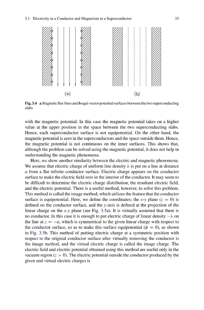
Fig. 3.4 a Magnetic flux lines and b equi-vector potential surfaces between the two superconducting
slabs
with the magnetic potential. In this case the magnetic potential takes on a higher
value at the upper position in the space between the two superconducting slabs.
Hence, each superconductor surface is not equipotential. On the other hand, the
magnetic potential is zero in the superconductors and the space outside them. Hence,
the magnetic potential is not continuous on the inner surfaces. This shows that,
although the problem can be solved using the magnetic potential, it does not help in
understanding the magnetic phenomena.
Here, we show another similarity between the electric and magnetic phenomena.
We assume that electric charge of uniform line density λ is put on a line at distance
a from a flat infinite conductor surface. Electric charge appears on the conductor
surface to make the electric field zero in the interior of the conductor. It may seem to
be difficult to determine the electric charge distribution, the resultant electric field,
and the electric potential. There is a useful method, however, to solve this problem.
This method is called the image method, which utilizes the feature that the conductor
surface is equipotential. Here, we define the coordinates; the x-y plane (z = 0) is
defined on the conductor surface, and the y-axis is defined at the projection of the
linear charge on the x-y plane (see Fig. 3.5a). It is virtually assumed that there is
no conductor. In this case it is enough to put electric charge of linear density −λ on
the line at z = −a, which is symmetrical to the given linear charge with respect to
the conductor surface, so as to make this surface equipotential (φ = 0), as shown
in Fig. 3.5b. This method of putting electric charge at a symmetric position with
respect to the original conductor surface after virtually removing the conductor is
the image method, and the virtual electric charge is called the image charge. The
electric field and electric potential obtained using this method are useful only in the
vacuum region (z > 0). The electric potential outside the conductor produced by the
given and virtual electric charges is
33
Fig. 3.4 a Magnetic flux lines and b equi-vector potential surfaces between the two superconducting
slabs
with the magnetic potential. In this case the magnetic potential takes on a higher
value at the upper position in the space between the two superconducting slabs.
Hence, each superconductor surface is not equipotential. On the other hand, the
magnetic potential is zero in the superconductors and the space outside them. Hence,
the magnetic potential is not continuous on the inner surfaces. This shows that,
although the problem can be solved using the magnetic potential, it does not help in
understanding the magnetic phenomena.
Here, we show another similarity between the electric and magnetic phenomena.
We assume that electric charge of uniform line density λ is put on a line at distance
a from a flat infinite conductor surface. Electric charge appears on the conductor
surface to make the electric field zero in the interior of the conductor. It may seem to
be difficult to determine the electric charge distribution, the resultant electric field,
and the electric potential. There is a useful method, however, to solve this problem.
This method is called the image method, which utilizes the feature that the conductor
surface is equipotential. Here, we define the coordinates; the x-y plane (z = 0) is
defined on the conductor surface, and the y-axis is defined at the projection of the
linear charge on the x-y plane (see Fig. 3.5a). It is virtually assumed that there is
no conductor. In this case it is enough to put electric charge of linear density −λ on
the line at z = −a, which is symmetrical to the given linear charge with respect to
the conductor surface, so as to make this surface equipotential (φ = 0), as shown
in Fig. 3.5b. This method of putting electric charge at a symmetric position with
respect to the original conductor surface after virtually removing the conductor is
the image method, and the virtual electric charge is called the image charge. The
electric field and electric potential obtained using this method are useful only in the
vacuum region (z > 0). The electric potential outside the conductor produced by the
given and virtual electric charges is