

120
6 Longitudinal Magnetic Field Effect
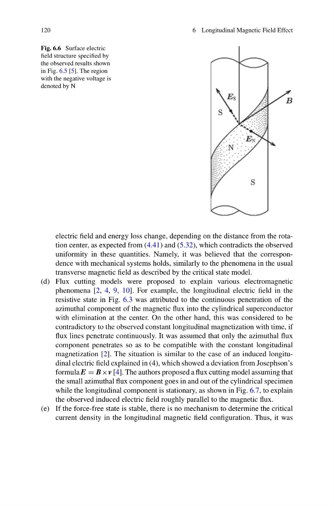
Fig. 6.6 Surface electric
field structure specified by
the observed results shown
in Fig. 6.5 [5]. The region
with the negative voltage is
denoted by N
electric field and energy loss change, depending on the distance from the rotation center, as expected from (4.41) and (5.32), which contradicts the observed
uniformity in these quantities. Namely, it was believed that the correspondence with mechanical systems holds, similarly to the phenomena in the usual
transverse magnetic field as described by the critical state model.
(d) Flux cutting models were proposed to explain various electromagnetic
phenomena [2, 4, 9, 10]. For example, the longitudinal electric field in the
resistive state in Fig. 6.3 was attributed to the continuous penetration of the
azimuthal component of the magnetic flux into the cylindrical superconductor
with elimination at the center. On the other hand, this was considered to be
contradictory to the observed constant longitudinal magnetization with time, if
flux lines penetrate continuously. It was assumed that only the azimuthal flux
component penetrates so as to be compatible with the constant longitudinal
magnetization [2]. The situation is similar to the case of an induced longitudinal electric field explained in (4), which showed a deviation from Josephson’s
formula E = B×v [4]. The authors proposed a flux cutting model assuming that
the small azimuthal flux component goes in and out of the cylindrical specimen
while the longitudinal component is stationary, as shown in Fig. 6.7, to explain
the observed induced electric field roughly parallel to the magnetic flux.
(e) If the force-free state is stable, there is no mechanism to determine the critical
current density in the longitudinal magnetic field configuration. Thus, it was
6 Longitudinal Magnetic Field Effect
Fig. 6.6 Surface electric
field structure specified by
the observed results shown
in Fig. 6.5 [5]. The region
with the negative voltage is
denoted by N
electric field and energy loss change, depending on the distance from the rotation center, as expected from (4.41) and (5.32), which contradicts the observed
uniformity in these quantities. Namely, it was believed that the correspondence with mechanical systems holds, similarly to the phenomena in the usual
transverse magnetic field as described by the critical state model.
(d) Flux cutting models were proposed to explain various electromagnetic
phenomena [2, 4, 9, 10]. For example, the longitudinal electric field in the
resistive state in Fig. 6.3 was attributed to the continuous penetration of the
azimuthal component of the magnetic flux into the cylindrical superconductor
with elimination at the center. On the other hand, this was considered to be
contradictory to the observed constant longitudinal magnetization with time, if
flux lines penetrate continuously. It was assumed that only the azimuthal flux
component penetrates so as to be compatible with the constant longitudinal
magnetization [2]. The situation is similar to the case of an induced longitudinal electric field explained in (4), which showed a deviation from Josephson’s
formula E = B×v [4]. The authors proposed a flux cutting model assuming that
the small azimuthal flux component goes in and out of the cylindrical specimen
while the longitudinal component is stationary, as shown in Fig. 6.7, to explain
the observed induced electric field roughly parallel to the magnetic flux.
(e) If the force-free state is stable, there is no mechanism to determine the critical
current density in the longitudinal magnetic field configuration. Thus, it was