

284 12 Characterization of Nanomaterials
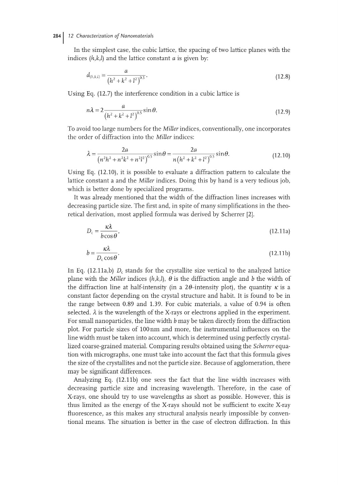
In the simplest case, the cubic lattice, the spacing of two lattice planes with the
indices (h,k,l) and the lattice constant a is given by:
d
a
h k l
h k l
, ,
. .
(
) =
+ +
(
)
2
2
2 0 5
(12.8)
Using Eq. (12.7) the interference condition in a cubic lattice is
n
a
h k l
λ
θ
=
+ +
(
)
2 2 2 2 0 5
. sin .
(12.9)
To avoid too large numbers for the Miller indices, conventionally, one incorporates
the order of diffraction into the Miller indices:
λ
θ
θ
=
+
+
(
)
=
+ +
(
)
2
2
2 2
2 2
2 2 0 5
2
2
2 0 5
a
n h n k n l
a
n h k l
.
.
.
sin
sin
(12.10)
Using Eq. (12.10), it is possible to evaluate a diffraction pattern to calculate the
lattice constant a and the Miller indices. Doing this by hand is a very tedious job,
which is better done by specialized programs.
It was already mentioned that the width of the diffraction lines increases with
decreasing particle size. The first and, in spite of many simplifications in the theoretical derivation, most applied formula was derived by Scherrer [2].
D b
c =
κλ
θ
cos
,
(12.11a)
b D
=
κλ
θ
c cos
.
(12.11b)
In Eq. (12.11a,b) D c stands for the crystallite size vertical to the analyzed lattice
plane with the Miller indices (h,k,l), θ is the diffraction angle and b the width of
the diffraction line at half-intensity (in a 2θ–intensity plot), the quantity κ is a
constant factor depending on the crystal structure and habit. It is found to be in
the range between 0.89 and 1.39. For cubic materials, a value of 0.94 is often
selected. λ is the wavelength of the X-rays or electrons applied in the experiment.
For small nanoparticles, the line width b may be taken directly from the diffraction
plot. For particle sizes of 100 nm and more, the instrumental influences on the
line width must be taken into account, which is determined using perfectly crystallized coarse-grained material. Comparing results obtained using the Scherrer equation with micrographs, one must take into account the fact that this formula gives
the size of the crystallites and not the particle size. Because of agglomeration, there
may be significant differences.
Analyzing Eq. (12.11b) one sees the fact that the line width increases with
decreasing particle size and increasing wavelength. Therefore, in the case of
X-rays, one should try to use wavelengths as short as possible. However, this is
thus limited as the energy of the X-rays should not be sufficient to excite X-ray
fluorescence, as this makes any structural analysis nearly impossible by conventional means. The situation is better in the case of electron diffraction. In this
In the simplest case, the cubic lattice, the spacing of two lattice planes with the
indices (h,k,l) and the lattice constant a is given by:
d
a
h k l
h k l
, ,
. .
(
) =
+ +
(
)
2
2
2 0 5
(12.8)
Using Eq. (12.7) the interference condition in a cubic lattice is
n
a
h k l
λ
θ
=
+ +
(
)
2 2 2 2 0 5
. sin .
(12.9)
To avoid too large numbers for the Miller indices, conventionally, one incorporates
the order of diffraction into the Miller indices:
λ
θ
θ
=
+
+
(
)
=
+ +
(
)
2
2
2 2
2 2
2 2 0 5
2
2
2 0 5
a
n h n k n l
a
n h k l
.
.
.
sin
sin
(12.10)
Using Eq. (12.10), it is possible to evaluate a diffraction pattern to calculate the
lattice constant a and the Miller indices. Doing this by hand is a very tedious job,
which is better done by specialized programs.
It was already mentioned that the width of the diffraction lines increases with
decreasing particle size. The first and, in spite of many simplifications in the theoretical derivation, most applied formula was derived by Scherrer [2].
D b
c =
κλ
θ
cos
,
(12.11a)
b D
=
κλ
θ
c cos
.
(12.11b)
In Eq. (12.11a,b) D c stands for the crystallite size vertical to the analyzed lattice
plane with the Miller indices (h,k,l), θ is the diffraction angle and b the width of
the diffraction line at half-intensity (in a 2θ–intensity plot), the quantity κ is a
constant factor depending on the crystal structure and habit. It is found to be in
the range between 0.89 and 1.39. For cubic materials, a value of 0.94 is often
selected. λ is the wavelength of the X-rays or electrons applied in the experiment.
For small nanoparticles, the line width b may be taken directly from the diffraction
plot. For particle sizes of 100 nm and more, the instrumental influences on the
line width must be taken into account, which is determined using perfectly crystallized coarse-grained material. Comparing results obtained using the Scherrer equation with micrographs, one must take into account the fact that this formula gives
the size of the crystallites and not the particle size. Because of agglomeration, there
may be significant differences.
Analyzing Eq. (12.11b) one sees the fact that the line width increases with
decreasing particle size and increasing wavelength. Therefore, in the case of
X-rays, one should try to use wavelengths as short as possible. However, this is
thus limited as the energy of the X-rays should not be sufficient to excite X-ray
fluorescence, as this makes any structural analysis nearly impossible by conventional means. The situation is better in the case of electron diffraction. In this