

246 10 Electrical Properties
the values are very close to nil. Therefore, again, as in the previous example, the
double-logarithmic plot according to Eq. (10.12) is presented.
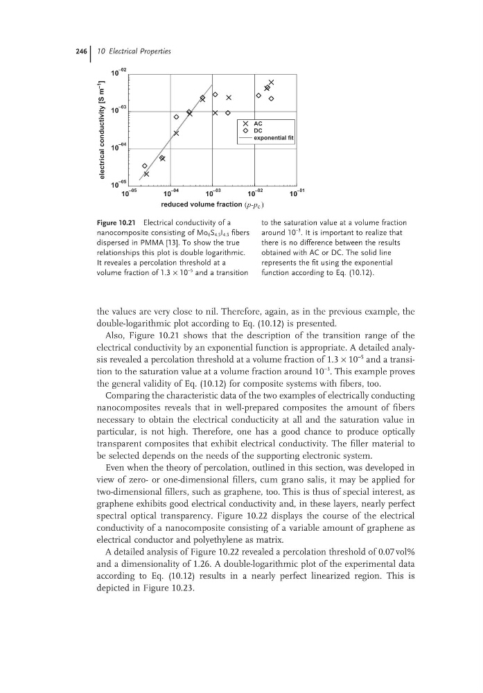
Also, Figure 10.21 shows that the description of the transition range of the
electrical conductivity by an exponential function is appropriate. A detailed analysis revealed a percolation threshold at a volume fraction of 1.3 × 10
−5 and a transition to the saturation value at a volume fraction around 10
−3 . This example proves
the general validity of Eq. (10.12) for composite systems with fibers, too.
Comparing the characteristic data of the two examples of electrically conducting
nanocomposites reveals that in well-prepared composites the amount of fibers
necessary to obtain the electrical conducticity at all and the saturation value in
particular, is not high. Therefore, one has a good chance to produce optically
transparent composites that exhibit electrical conductivity. The filler material to
be selected depends on the needs of the supporting electronic system.
Even when the theory of percolation, outlined in this section, was developed in
view of zero- or one-dimensional fillers, cum grano salis, it may be applied for
two-dimensional fillers, such as graphene, too. This is thus of special interest, as
graphene exhibits good electrical conductivity and, in these layers, nearly perfect
spectral optical transparency. Figure 10.22 displays the course of the electrical
conductivity of a nanocomposite consisting of a variable amount of graphene as
electrical conductor and polyethylene as matrix.
A detailed analysis of Figure 10.22 revealed a percolation threshold of 0.07 vol%
and a dimensionality of 1.26. A double-logarithmic plot of the experimental data
according to Eq. (10.12) results in a nearly perfect linearized region. This is
depicted in Figure 10.23.
Figure 10.21 Electrical conductivity of a
nanocomposite consisting of Mo 6 S 4.5 I 4.5 fibers
dispersed in PMMA [13]. To show the true
relationships this plot is double logarithmic.
It reveales a percolation threshold at a
volume fraction of 1.3 × 10
−5 and a transition
to the saturation value at a volume fraction
around 10
−3 . It is important to realize that
there is no difference between the results
obtained with AC or DC. The solid line
represents the fit using the exponential
function according to Eq. (10.12).
10
–05
10
–04
10
–03
10
–02
10
–01
reduced volume fraction (p-p c )
10
–05
10
–04
10
–03
10
–02
electrical
conductivity
[S
m
–1
]
AC
DC
exponential fit
the values are very close to nil. Therefore, again, as in the previous example, the
double-logarithmic plot according to Eq. (10.12) is presented.
Also, Figure 10.21 shows that the description of the transition range of the
electrical conductivity by an exponential function is appropriate. A detailed analysis revealed a percolation threshold at a volume fraction of 1.3 × 10
−5 and a transition to the saturation value at a volume fraction around 10
−3 . This example proves
the general validity of Eq. (10.12) for composite systems with fibers, too.
Comparing the characteristic data of the two examples of electrically conducting
nanocomposites reveals that in well-prepared composites the amount of fibers
necessary to obtain the electrical conducticity at all and the saturation value in
particular, is not high. Therefore, one has a good chance to produce optically
transparent composites that exhibit electrical conductivity. The filler material to
be selected depends on the needs of the supporting electronic system.
Even when the theory of percolation, outlined in this section, was developed in
view of zero- or one-dimensional fillers, cum grano salis, it may be applied for
two-dimensional fillers, such as graphene, too. This is thus of special interest, as
graphene exhibits good electrical conductivity and, in these layers, nearly perfect
spectral optical transparency. Figure 10.22 displays the course of the electrical
conductivity of a nanocomposite consisting of a variable amount of graphene as
electrical conductor and polyethylene as matrix.
A detailed analysis of Figure 10.22 revealed a percolation threshold of 0.07 vol%
and a dimensionality of 1.26. A double-logarithmic plot of the experimental data
according to Eq. (10.12) results in a nearly perfect linearized region. This is
depicted in Figure 10.23.
Figure 10.21 Electrical conductivity of a
nanocomposite consisting of Mo 6 S 4.5 I 4.5 fibers
dispersed in PMMA [13]. To show the true
relationships this plot is double logarithmic.
It reveales a percolation threshold at a
volume fraction of 1.3 × 10
−5 and a transition
to the saturation value at a volume fraction
around 10
−3 . It is important to realize that
there is no difference between the results
obtained with AC or DC. The solid line
represents the fit using the exponential
function according to Eq. (10.12).
10
–05
10
–04
10
–03
10
–02
10
–01
reduced volume fraction (p-p c )
10
–05
10
–04
10
–03
10
–02
electrical
conductivity
[S
m
–1
]
AC
DC
exponential fit