

8.2 Fundamentals of Superparamagnetism 157
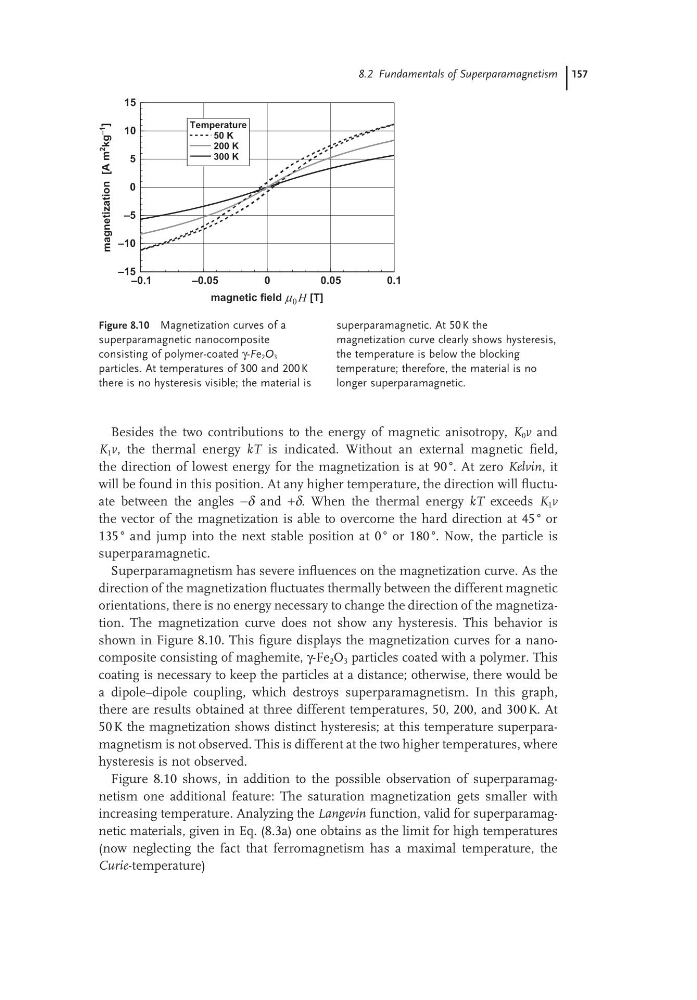
Figure 8.10 Magnetization curves of a
superparamagnetic nanocomposite
consisting of polymer-coated γ-Fe 2 O 3
particles. At temperatures of 300 and 200 K
there is no hysteresis visible; the material is
superparamagnetic. At 50 K the
magnetization curve clearly shows hysteresis,
the temperature is below the blocking
temperature; therefore, the material is no
longer superparamagnetic.
–0.1
–0.05
0
0.05
0.1
magnetic field µ 0 H [T]
–15
–10
–5
0
5
10
15
magnetization
[A
m
2
kg
–1
]
Temperature
50 K
200 K
300 K
Besides the two contributions to the energy of magnetic anisotropy, K 0 v and
K 1 v, the thermal energy kT is indicated. Without an external magnetic field,
the direction of lowest energy for the magnetization is at 90 °. At zero Kelvin, it
will be found in this position. At any higher temperature, the direction will fluctuate between the angles −δ and +δ. When the thermal energy kT exceeds K 1 v
the vector of the magnetization is able to overcome the hard direction at 45 ° or
135 ° and jump into the next stable position at 0 ° or 180 °. Now, the particle is
superparamagnetic.
Superparamagnetism has severe influences on the magnetization curve. As the
direction of the magnetization fluctuates thermally between the different magnetic
orientations, there is no energy necessary to change the direction of the magnetization. The magnetization curve does not show any hysteresis. This behavior is
shown in Figure 8.10. This figure displays the magnetization curves for a nanocomposite consisting of maghemite, γFe 2 O 3 particles coated with a polymer. This
coating is necessary to keep the particles at a distance; otherwise, there would be
a dipole–dipole coupling, which destroys superparamagnetism. In this graph,
there are results obtained at three different temperatures, 50, 200, and 300 K. At
50 K the magnetization shows distinct hysteresis; at this temperature superparamagnetism is not observed. This is different at the two higher temperatures, where
hysteresis is not observed.
Figure 8.10 shows, in addition to the possible observation of superparamagnetism one additional feature: The saturation magnetization gets smaller with
increasing temperature. Analyzing the Langevin function, valid for superparamagnetic materials, given in Eq. (8.3a) one obtains as the limit for high temperatures
(now neglecting the fact that ferromagnetism has a maximal temperature, the
Curietemperature)
Figure 8.10 Magnetization curves of a
superparamagnetic nanocomposite
consisting of polymer-coated γ-Fe 2 O 3
particles. At temperatures of 300 and 200 K
there is no hysteresis visible; the material is
superparamagnetic. At 50 K the
magnetization curve clearly shows hysteresis,
the temperature is below the blocking
temperature; therefore, the material is no
longer superparamagnetic.
–0.1
–0.05
0
0.05
0.1
magnetic field µ 0 H [T]
–15
–10
–5
0
5
10
15
magnetization
[A
m
2
kg
–1
]
Temperature
50 K
200 K
300 K
Besides the two contributions to the energy of magnetic anisotropy, K 0 v and
K 1 v, the thermal energy kT is indicated. Without an external magnetic field,
the direction of lowest energy for the magnetization is at 90 °. At zero Kelvin, it
will be found in this position. At any higher temperature, the direction will fluctuate between the angles −δ and +δ. When the thermal energy kT exceeds K 1 v
the vector of the magnetization is able to overcome the hard direction at 45 ° or
135 ° and jump into the next stable position at 0 ° or 180 °. Now, the particle is
superparamagnetic.
Superparamagnetism has severe influences on the magnetization curve. As the
direction of the magnetization fluctuates thermally between the different magnetic
orientations, there is no energy necessary to change the direction of the magnetization. The magnetization curve does not show any hysteresis. This behavior is
shown in Figure 8.10. This figure displays the magnetization curves for a nanocomposite consisting of maghemite, γFe 2 O 3 particles coated with a polymer. This
coating is necessary to keep the particles at a distance; otherwise, there would be
a dipole–dipole coupling, which destroys superparamagnetism. In this graph,
there are results obtained at three different temperatures, 50, 200, and 300 K. At
50 K the magnetization shows distinct hysteresis; at this temperature superparamagnetism is not observed. This is different at the two higher temperatures, where
hysteresis is not observed.
Figure 8.10 shows, in addition to the possible observation of superparamagnetism one additional feature: The saturation magnetization gets smaller with
increasing temperature. Analyzing the Langevin function, valid for superparamagnetic materials, given in Eq. (8.3a) one obtains as the limit for high temperatures
(now neglecting the fact that ferromagnetism has a maximal temperature, the
Curietemperature)