

Epoxy Molecular Structure Alteration in Graphene …
469
The physical mechanisms underlying loading-induced evolution of an ensemble of
the γ -dipoles populating 3D-molecular architecture of the epoxy resin can be ascertained by using theoretical modeling of dependences of ε 2 versus ε 1 . It is clearly seen
from Fig. 5, that the experimental locuses are very close to circular ones. A careful
geometric analysis of the locuses by using the Havriliak–Negami fitting procedure
[72] shows that the Havriliak–Negami model’s parameter β has proven to be greater
than unity. In other words, the Havriliak–Negami model fails to comprehend the
experimental data. Therefore, the Cole–Cole model has been used. The solid lines
given on Fig. 5 have been calculated by using the relation [53]:
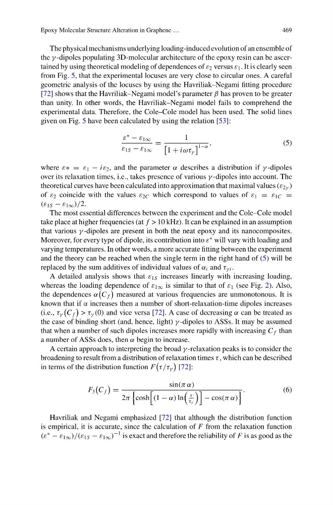
ε
∗
− ε 1∞
ε 1S − ε 1∞
=
1
1 + iωτ γ
1−α ,
(5)
where ε∗ = ε 1 − iε 2 , and the parameter α describes a distribution if γ -dipoles
over its relaxation times, i.e., takes presence of various γ -dipoles into account. The
theoretical curves have been calculated into approximation that maximal values (ε 2γ )
of ε 2 coincide with the values ε 2C which correspond to values of ε 1 = ε 1C =
(ε 1S − ε 1∞ )/2.
The most essential differences between the experiment and the Cole–Cole model
take place at higher frequencies (at f > 10 kHz). It can be explained in an assumption
that various γ -dipoles are present in both the neat epoxy and its nanocomposites.
Moreover, for every type of dipole, its contribution into ε
∗ will vary with loading and
varying temperatures. In other words, a more accurate fitting between the experiment
and the theory can be reached when the single term in the right hand of (5) will be
replaced by the sum additives of individual values of α i and τ γ i .
A detailed analysis shows that ε 1S increases linearly with increasing loading,
whereas the loading dependence of ε 1∞ is similar to that of ε 1 (see Fig. 2). Also,
the dependences α
C f
measured at various frequencies are unmonotonous. It is
known that if α increases then a number of short-relaxation-time dipoles increases
(i.e., τ γ
C f
> τ γ (0) and vice versa [72]. A case of decreasing α can be treated as
the case of binding short (and, hence, light) γ -dipoles to ASSs. It may be assumed
that when a number of such dipoles increases more rapidly with increasing C f than
a number of ASSs does, then α begin to increase.
A certain approach to interpreting the broad γ -relaxation peaks is to consider the
broadening to result from a distribution of relaxation times τ , which can be described
in terms of the distribution function F
τ/τ γ
[72]:
F 3
C f
=
sin(π α)
2π
cosh
(1 − α) ln
τ
τ γ
− cos(π α)
.
(6)
Havriliak and Negami emphasized [72] that although the distribution function
is empirical, it is accurate, since the calculation of F from the relaxation function
(ε
∗
− ε 1∞ )/(ε 1S − ε 1∞ )
−1 is exact and therefore the reliability of F is as good as the
469
The physical mechanisms underlying loading-induced evolution of an ensemble of
the γ -dipoles populating 3D-molecular architecture of the epoxy resin can be ascertained by using theoretical modeling of dependences of ε 2 versus ε 1 . It is clearly seen
from Fig. 5, that the experimental locuses are very close to circular ones. A careful
geometric analysis of the locuses by using the Havriliak–Negami fitting procedure
[72] shows that the Havriliak–Negami model’s parameter β has proven to be greater
than unity. In other words, the Havriliak–Negami model fails to comprehend the
experimental data. Therefore, the Cole–Cole model has been used. The solid lines
given on Fig. 5 have been calculated by using the relation [53]:
ε
∗
− ε 1∞
ε 1S − ε 1∞
=
1
1 + iωτ γ
1−α ,
(5)
where ε∗ = ε 1 − iε 2 , and the parameter α describes a distribution if γ -dipoles
over its relaxation times, i.e., takes presence of various γ -dipoles into account. The
theoretical curves have been calculated into approximation that maximal values (ε 2γ )
of ε 2 coincide with the values ε 2C which correspond to values of ε 1 = ε 1C =
(ε 1S − ε 1∞ )/2.
The most essential differences between the experiment and the Cole–Cole model
take place at higher frequencies (at f > 10 kHz). It can be explained in an assumption
that various γ -dipoles are present in both the neat epoxy and its nanocomposites.
Moreover, for every type of dipole, its contribution into ε
∗ will vary with loading and
varying temperatures. In other words, a more accurate fitting between the experiment
and the theory can be reached when the single term in the right hand of (5) will be
replaced by the sum additives of individual values of α i and τ γ i .
A detailed analysis shows that ε 1S increases linearly with increasing loading,
whereas the loading dependence of ε 1∞ is similar to that of ε 1 (see Fig. 2). Also,
the dependences α
C f
measured at various frequencies are unmonotonous. It is
known that if α increases then a number of short-relaxation-time dipoles increases
(i.e., τ γ
C f
> τ γ (0) and vice versa [72]. A case of decreasing α can be treated as
the case of binding short (and, hence, light) γ -dipoles to ASSs. It may be assumed
that when a number of such dipoles increases more rapidly with increasing C f than
a number of ASSs does, then α begin to increase.
A certain approach to interpreting the broad γ -relaxation peaks is to consider the
broadening to result from a distribution of relaxation times τ , which can be described
in terms of the distribution function F
τ/τ γ
[72]:
F 3
C f
=
sin(π α)
2π
cosh
(1 − α) ln
τ
τ γ
− cos(π α)
.
(6)
Havriliak and Negami emphasized [72] that although the distribution function
is empirical, it is accurate, since the calculation of F from the relaxation function
(ε
∗
− ε 1∞ )/(ε 1S − ε 1∞ )
−1 is exact and therefore the reliability of F is as good as the