

New Effective Filter in the Spatial Domain for Speckle Noise Reduction
183
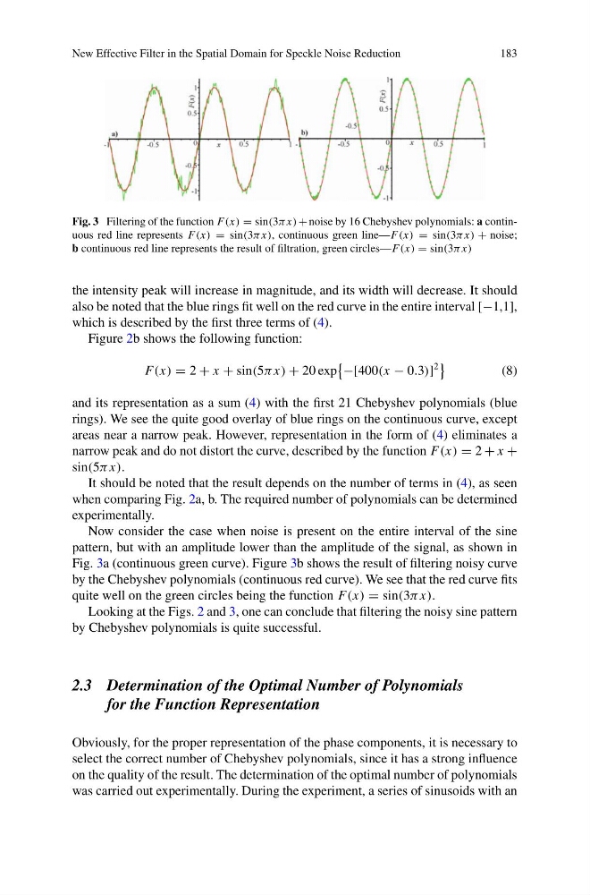
Fig. 3 Filtering of the function F(x) = sin(3π x) + noise by 16 Chebyshev polynomials: a continuous red line represents F(x) = sin(3π x), continuous green line—F(x) = sin(3π x) + noise;
b continuous red line represents the result of filtration, green circles—F(x) = sin(3π x)
the intensity peak will increase in magnitude, and its width will decrease. It should
also be noted that the blue rings fit well on the red curve in the entire interval [−1,1],
which is described by the first three terms of (4).
Figure 2b shows the following function:
F(x) = 2 + x + sin(5π x) + 20 exp
−[400(x − 0.3)]
2
(8)
and its representation as a sum (4) with the first 21 Chebyshev polynomials (blue
rings). We see the quite good overlay of blue rings on the continuous curve, except
areas near a narrow peak. However, representation in the form of (4) eliminates a
narrow peak and do not distort the curve, described by the function F(x) = 2 + x +
sin(5π x).
It should be noted that the result depends on the number of terms in (4), as seen
when comparing Fig. 2a, b. The required number of polynomials can be determined
experimentally.
Now consider the case when noise is present on the entire interval of the sine
pattern, but with an amplitude lower than the amplitude of the signal, as shown in
Fig. 3a (continuous green curve). Figure 3b shows the result of filtering noisy curve
by the Chebyshev polynomials (continuous red curve). We see that the red curve fits
quite well on the green circles being the function F(x) = sin(3π x).
Looking at the Figs. 2 and 3, one can conclude that filtering the noisy sine pattern
by Chebyshev polynomials is quite successful.
2.3 Determination of the Optimal Number of Polynomials
for the Function Representation
Obviously, for the proper representation of the phase components, it is necessary to
select the correct number of Chebyshev polynomials, since it has a strong influence
on the quality of the result. The determination of the optimal number of polynomials
was carried out experimentally. During the experiment, a series of sinusoids with an
183
Fig. 3 Filtering of the function F(x) = sin(3π x) + noise by 16 Chebyshev polynomials: a continuous red line represents F(x) = sin(3π x), continuous green line—F(x) = sin(3π x) + noise;
b continuous red line represents the result of filtration, green circles—F(x) = sin(3π x)
the intensity peak will increase in magnitude, and its width will decrease. It should
also be noted that the blue rings fit well on the red curve in the entire interval [−1,1],
which is described by the first three terms of (4).
Figure 2b shows the following function:
F(x) = 2 + x + sin(5π x) + 20 exp
−[400(x − 0.3)]
2
(8)
and its representation as a sum (4) with the first 21 Chebyshev polynomials (blue
rings). We see the quite good overlay of blue rings on the continuous curve, except
areas near a narrow peak. However, representation in the form of (4) eliminates a
narrow peak and do not distort the curve, described by the function F(x) = 2 + x +
sin(5π x).
It should be noted that the result depends on the number of terms in (4), as seen
when comparing Fig. 2a, b. The required number of polynomials can be determined
experimentally.
Now consider the case when noise is present on the entire interval of the sine
pattern, but with an amplitude lower than the amplitude of the signal, as shown in
Fig. 3a (continuous green curve). Figure 3b shows the result of filtering noisy curve
by the Chebyshev polynomials (continuous red curve). We see that the red curve fits
quite well on the green circles being the function F(x) = sin(3π x).
Looking at the Figs. 2 and 3, one can conclude that filtering the noisy sine pattern
by Chebyshev polynomials is quite successful.
2.3 Determination of the Optimal Number of Polynomials
for the Function Representation
Obviously, for the proper representation of the phase components, it is necessary to
select the correct number of Chebyshev polynomials, since it has a strong influence
on the quality of the result. The determination of the optimal number of polynomials
was carried out experimentally. During the experiment, a series of sinusoids with an