

132
L. Didukh et al.
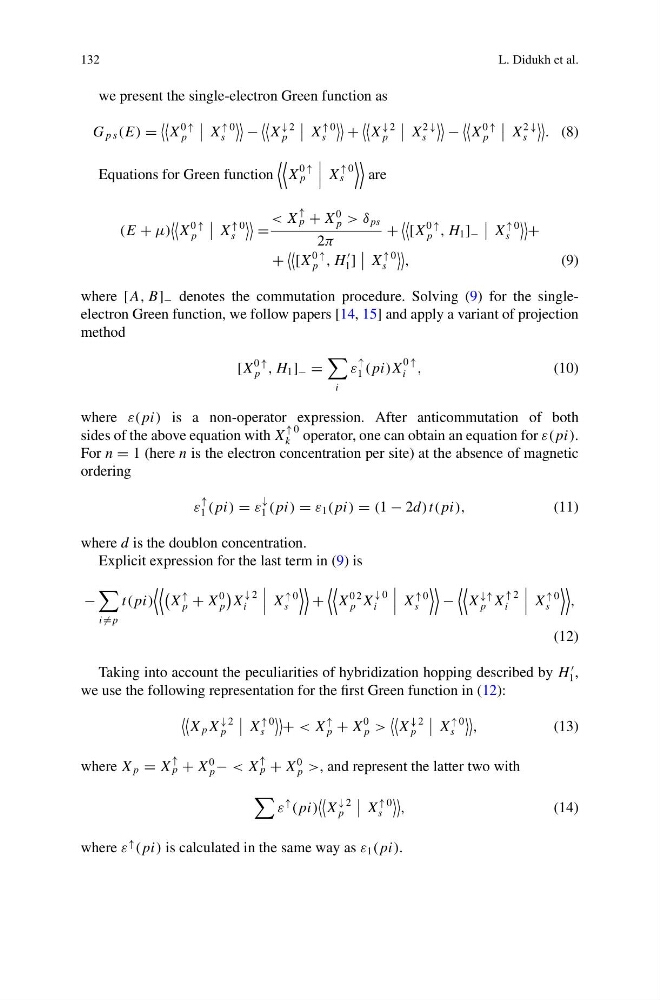
we present the single-electron Green function as
G p s (E) =
X
0 ↑
p
X
↑ 0
s
−
X
↓ 2
p
X
↑ 0
s
+
X
↓ 2
p
X
2 ↓
s
−
X
0 ↑
p
X
2 ↓
s
. (8)
Equations for Green function
X
0 ↑
p
X
↑ 0
s
are
(E + μ)
X
0 ↑
p
X
↑ 0
s
=
< X
↑
p + X
0
p > δ ps
2π
+
[X
0 ↑
p , H 1 ] −
X
↑ 0
s
+
+
[X
0 ↑
p , H
1 ]
X
↑ 0
s
,
(9)
where [A, B] − denotes the commutation procedure. Solving (9) for the singleelectron Green function, we follow papers [14, 15] and apply a variant of projection
method
[X
0 ↑
p , H 1 ] − =
i
ε
↑
1 ( pi)X
0 ↑
i ,
(10)
where ε( pi) is a non-operator expression. After anticommutation of both
sides of the above equation with X
↑ 0
k operator, one can obtain an equation for ε( pi).
For n = 1 (here n is the electron concentration per site) at the absence of magnetic
ordering
ε
↑
1 ( pi) = ε
↓
1 ( pi) = ε 1 ( pi) = (1 − 2d)t( pi),
(11)
where d is the doublon concentration.
Explicit expression for the last term in (9) is
−
i = p
t( pi)
X
↑
p + X
0
p
X
↓ 2
i
X
↑ 0
s
+
X
0 2
p X
↓ 0
i
X
↑ 0
s
−
X
↓↑
p X
↑ 2
i
X
↑ 0
s
,
(12)
Taking into account the peculiarities of hybridization hopping described by H
1 ,
we use the following representation for the first Green function in (12):
X p X
↓ 2
p
X
↑ 0
s
+ < X
↑
p + X
0
p >
X
↓ 2
p
X
↑ 0
s
,
(13)
where X p = X
↑
p + X
0
p − < X
↑
p + X
0
p >, and represent the latter two with
ε
↑
( pi)
X
↓ 2
p
X
↑ 0
s
,
(14)
where ε
↑
( pi) is calculated in the same way as ε 1 ( pi).
L. Didukh et al.
we present the single-electron Green function as
G p s (E) =
X
0 ↑
p
X
↑ 0
s
−
X
↓ 2
p
X
↑ 0
s
+
X
↓ 2
p
X
2 ↓
s
−
X
0 ↑
p
X
2 ↓
s
. (8)
Equations for Green function
X
0 ↑
p
X
↑ 0
s
are
(E + μ)
X
0 ↑
p
X
↑ 0
s
=
< X
↑
p + X
0
p > δ ps
2π
+
[X
0 ↑
p , H 1 ] −
X
↑ 0
s
+
+
[X
0 ↑
p , H
1 ]
X
↑ 0
s
,
(9)
where [A, B] − denotes the commutation procedure. Solving (9) for the singleelectron Green function, we follow papers [14, 15] and apply a variant of projection
method
[X
0 ↑
p , H 1 ] − =
i
ε
↑
1 ( pi)X
0 ↑
i ,
(10)
where ε( pi) is a non-operator expression. After anticommutation of both
sides of the above equation with X
↑ 0
k operator, one can obtain an equation for ε( pi).
For n = 1 (here n is the electron concentration per site) at the absence of magnetic
ordering
ε
↑
1 ( pi) = ε
↓
1 ( pi) = ε 1 ( pi) = (1 − 2d)t( pi),
(11)
where d is the doublon concentration.
Explicit expression for the last term in (9) is
−
i = p
t( pi)
X
↑
p + X
0
p
X
↓ 2
i
X
↑ 0
s
+
X
0 2
p X
↓ 0
i
X
↑ 0
s
−
X
↓↑
p X
↑ 2
i
X
↑ 0
s
,
(12)
Taking into account the peculiarities of hybridization hopping described by H
1 ,
we use the following representation for the first Green function in (12):
X p X
↓ 2
p
X
↑ 0
s
+ < X
↑
p + X
0
p >
X
↓ 2
p
X
↑ 0
s
,
(13)
where X p = X
↑
p + X
0
p − < X
↑
p + X
0
p >, and represent the latter two with
ε
↑
( pi)
X
↓ 2
p
X
↑ 0
s
,
(14)
where ε
↑
( pi) is calculated in the same way as ε 1 ( pi).