

Modified Two-Pole Approximation for Systems with Strong Electron Correlations …
133
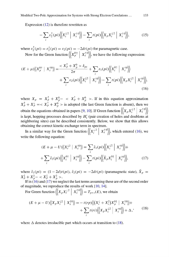
Expression (12) is therefore rewritten as
−
i
ε
↑
2 ( pi)
X
↓ 2
i
X
↑ 0
s
−
i
t( pi)
X p X
↓ 2
i
X
↑ 0
s
,
(15)
where ε
↑
2 ( pi) = ε
↓
2 ( pi) = ε 2 ( pi) = −2dt( pi) for paramagnetic case.
Now for the Green function
X
0 ↑
p
X
↑ 0
s
, we have the following expression:
(E + μ)
X
0↑
p
X
↑0
s
=
< X
↑
p + X
0
p > δ ps
2π
+
i
ε 1 ( pi)
X
0↑
i
X
↑0
s
+
i
ε 2 ( pi)
X
↓2
i
X
↑0
s
−
i
t( pi)
X p X
↓2
i
X
↑0
s
,
(16)
where X p = X
↑
p + X
0
p − < X
↑
p + X
0
p >. If in this equation approximation
X
↑
p + X
↓
p =< X
↑
p + X
0
p > is adopted (the last Green function is absent), then we
obtain the equations obtained in papers [9, 10]. If Green function
X p X
↓ 2
i
X
↑ 0
s
is kept, hopping processes described by H
1 (pair creation of holes and doublons at
neighboring sites) can be described consistently. Below, we show that this allows
obtaining the correct kinetic exchange term in spectrum.
In a similar way for the Green function
X
↓ 2
i
X
↑ 0
s
, which entered (16), we
write the following equation:
(E + μ − U )
X
↓2
r
X
↑0
s
=
i
˜
ε 1 ( pi)
X
↓2
i
X
↑0
s
+
+
i
˜
ε 2 ( pi)
X
0↑
i
X
↑0
s
−
i
t( pi)
˜
X p X
0↑
i
X
↑0
s
,
(17)
where ˜
ε 1 ( pi) = (1 − 2d)t( pi), ˜
ε 2 ( pi) = −2dt( pi) (paramagnetic state), ˜
X p =
X
↓
p + X
2
p − < X
↓
p + X
2
p >.
If in (16) and (17) we neglect the last terms assuming these are of the second order
of magnitude, we reproduce the results of work [10, 14].
For Green function
X p X
↓ 2
r
X
↑ 0
s
= T p r s (E), we obtain
(E + μ − U )
X p X
↓2
r
X
↑0
s
= − t(r p)
X
↓
r + X
2
r
X
0↑
p
X
↑0
s
+
+
i
t(ri)
X p X
↓2
i
X
↑0
s
+ ,
,
(18)
where denotes irreducible part which occurs at transition to (18).
133
Expression (12) is therefore rewritten as
−
i
ε
↑
2 ( pi)
X
↓ 2
i
X
↑ 0
s
−
i
t( pi)
X p X
↓ 2
i
X
↑ 0
s
,
(15)
where ε
↑
2 ( pi) = ε
↓
2 ( pi) = ε 2 ( pi) = −2dt( pi) for paramagnetic case.
Now for the Green function
X
0 ↑
p
X
↑ 0
s
, we have the following expression:
(E + μ)
X
0↑
p
X
↑0
s
=
< X
↑
p + X
0
p > δ ps
2π
+
i
ε 1 ( pi)
X
0↑
i
X
↑0
s
+
i
ε 2 ( pi)
X
↓2
i
X
↑0
s
−
i
t( pi)
X p X
↓2
i
X
↑0
s
,
(16)
where X p = X
↑
p + X
0
p − < X
↑
p + X
0
p >. If in this equation approximation
X
↑
p + X
↓
p =< X
↑
p + X
0
p > is adopted (the last Green function is absent), then we
obtain the equations obtained in papers [9, 10]. If Green function
X p X
↓ 2
i
X
↑ 0
s
is kept, hopping processes described by H
1 (pair creation of holes and doublons at
neighboring sites) can be described consistently. Below, we show that this allows
obtaining the correct kinetic exchange term in spectrum.
In a similar way for the Green function
X
↓ 2
i
X
↑ 0
s
, which entered (16), we
write the following equation:
(E + μ − U )
X
↓2
r
X
↑0
s
=
i
˜
ε 1 ( pi)
X
↓2
i
X
↑0
s
+
+
i
˜
ε 2 ( pi)
X
0↑
i
X
↑0
s
−
i
t( pi)
˜
X p X
0↑
i
X
↑0
s
,
(17)
where ˜
ε 1 ( pi) = (1 − 2d)t( pi), ˜
ε 2 ( pi) = −2dt( pi) (paramagnetic state), ˜
X p =
X
↓
p + X
2
p − < X
↓
p + X
2
p >.
If in (16) and (17) we neglect the last terms assuming these are of the second order
of magnitude, we reproduce the results of work [10, 14].
For Green function
X p X
↓ 2
r
X
↑ 0
s
= T p r s (E), we obtain
(E + μ − U )
X p X
↓2
r
X
↑0
s
= − t(r p)
X
↓
r + X
2
r
X
0↑
p
X
↑0
s
+
+
i
t(ri)
X p X
↓2
i
X
↑0
s
+ ,
,
(18)
where denotes irreducible part which occurs at transition to (18).