

3.2 Eigenvalue Problem
59
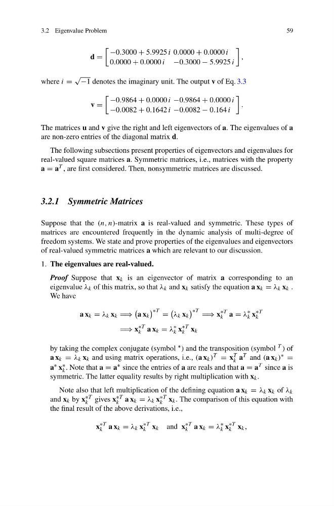
d =
−0.3000 + 5.9925 i 0.0000 + 0.0000 i
0.0000 + 0.0000 i −0.3000 − 5.9925 i
,
where i =
√ −1 denotes the imaginary unit. The output v of Eq. 3.3
v =
−0.9864 + 0.0000 i −0.9864 + 0.0000 i
−0.0082 + 0.1642 i −0.0082 − 0.164 i
.
The matrices u and v give the right and left eigenvectors of a. The eigenvalues of a
are non-zero entries of the diagonal matrix d.
The following subsections present properties of eigenvectors and eigenvalues for
real-valued square matrices a. Symmetric matrices, i.e., matrices with the property
a = a T , are first considered. Then, nonsymmetric matrices are discussed.
3.2.1 Symmetric Matrices
Suppose that the (n, n)-matrix a is real-valued and symmetric. These types of
matrices are encountered frequently in the dynamic analysis of multi-degree of
freedom systems. We state and prove properties of the eigenvalues and eigenvectors
of real-valued symmetric matrices a which are relevant to our discussion.
1. The eigenvalues are real-valued.
Proof Suppose that x k is an eigenvector of matrix a corresponding to an
eigenvalue λ k of this matrix, so that λ k and x k satisfy the equation a x k = λ k x k .
We have
a x k = λ k x k ⇒
a x k
∗T =
λ k x k
∗T ⇒ x
∗T
k a = λ
∗
k x
∗T
k
⇒ x
∗T
k a x k = λ
∗
k x
∗T
k x k
by taking the complex conjugate (symbol ∗ ) and the transposition (symbol T ) of
a x k = λ k x k and using matrix operations, i.e., (a x k ) T = x T
k a T and (a x k ) ∗ =
a ∗ x ∗
k . Note that a = a ∗ since the entries of a are reals and that a = a T since a is
symmetric. The latter equality results by right multiplication with x k .
Note also that left multiplication of the defining equation a x k = λ k x k of λ k
and x k by x ∗T
k gives x ∗T
k a x k = λ k x ∗T
k x k . The comparison of this equation with
the final result of the above derivations, i.e.,
x
∗T
k a x k = λ k x
∗T
k x k and x
∗T
k a x k = λ
∗
k x
∗T
k x k ,
59
d =
−0.3000 + 5.9925 i 0.0000 + 0.0000 i
0.0000 + 0.0000 i −0.3000 − 5.9925 i
,
where i =
√ −1 denotes the imaginary unit. The output v of Eq. 3.3
v =
−0.9864 + 0.0000 i −0.9864 + 0.0000 i
−0.0082 + 0.1642 i −0.0082 − 0.164 i
.
The matrices u and v give the right and left eigenvectors of a. The eigenvalues of a
are non-zero entries of the diagonal matrix d.
The following subsections present properties of eigenvectors and eigenvalues for
real-valued square matrices a. Symmetric matrices, i.e., matrices with the property
a = a T , are first considered. Then, nonsymmetric matrices are discussed.
3.2.1 Symmetric Matrices
Suppose that the (n, n)-matrix a is real-valued and symmetric. These types of
matrices are encountered frequently in the dynamic analysis of multi-degree of
freedom systems. We state and prove properties of the eigenvalues and eigenvectors
of real-valued symmetric matrices a which are relevant to our discussion.
1. The eigenvalues are real-valued.
Proof Suppose that x k is an eigenvector of matrix a corresponding to an
eigenvalue λ k of this matrix, so that λ k and x k satisfy the equation a x k = λ k x k .
We have
a x k = λ k x k ⇒
a x k
∗T =
λ k x k
∗T ⇒ x
∗T
k a = λ
∗
k x
∗T
k
⇒ x
∗T
k a x k = λ
∗
k x
∗T
k x k
by taking the complex conjugate (symbol ∗ ) and the transposition (symbol T ) of
a x k = λ k x k and using matrix operations, i.e., (a x k ) T = x T
k a T and (a x k ) ∗ =
a ∗ x ∗
k . Note that a = a ∗ since the entries of a are reals and that a = a T since a is
symmetric. The latter equality results by right multiplication with x k .
Note also that left multiplication of the defining equation a x k = λ k x k of λ k
and x k by x ∗T
k gives x ∗T
k a x k = λ k x ∗T
k x k . The comparison of this equation with
the final result of the above derivations, i.e.,
x
∗T
k a x k = λ k x
∗T
k x k and x
∗T
k a x k = λ
∗
k x
∗T
k x k ,