

58
3 Eigenvalue Problem
MATLAB Calculation of Eigenvalues/Eigenvectors Hand calculations using
Eqs. 3.1 and 3.2 are feasible for small-dimensional matrices. It is preferable to find
the eigenvalues and eigenvectors of a by MATLAB from
[u, d] = eig(a) (symmetric matrices)
[u, d] = eig(a) and [v, d] = eig(a
) (nonsymmetric matrices),
(3.3)
where u, v, and d are (n, n)-matrices and the notation a indicates matrix transposition in MATLAB. The columns of u in the first call are the eigenvectors of
symmetric matrices a. The columns of u and v in the second call are the right
and left eigenvectors of nonsymmetric matrices a. The diagonal matrix d gives the
eigenvalues of a, which coincide with those of a T . The columns of u and v are
aligned with those of d, e.g., column r of u and v and column r of d correspond to
the eigenvalue-eigenvector pair r.
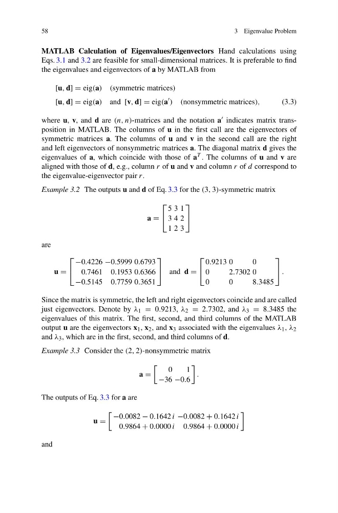
Example 3.2 The outputs u and d of Eq. 3.3 for the (3, 3)-symmetric matrix
a =
⎡
⎣
5 3 1
3 4 2
1 2 3
⎤
⎦
are
u =
⎡
⎣
−0.4226 −0.5999 0.6793
0.7461 0.1953 0.6366
−0.5145 0.7759 0.3651
⎤
⎦ and d =
⎡
⎣
0.9213 0
0
0
2.7302 0
0
0
8.3485
⎤
⎦ .
Since the matrix is symmetric, the left and right eigenvectors coincide and are called
just eigenvectors. Denote by λ 1 = 0.9213, λ 2 = 2.7302, and λ 3 = 8.3485 the
eigenvalues of this matrix. The first, second, and third columns of the MATLAB
output u are the eigenvectors x 1 , x 2 , and x 3 associated with the eigenvalues λ 1 , λ 2
and λ 3 , which are in the first, second, and third columns of d.
Example 3.3 Consider the (2, 2)-nonsymmetric matrix
a =
0
1
−36 −0.6
.
The outputs of Eq. 3.3 for a are
u =
−0.0082 − 0.1642 i −0.0082 + 0.1642 i
0.9864 + 0.0000 i 0.9864 + 0.0000 i
and
3 Eigenvalue Problem
MATLAB Calculation of Eigenvalues/Eigenvectors Hand calculations using
Eqs. 3.1 and 3.2 are feasible for small-dimensional matrices. It is preferable to find
the eigenvalues and eigenvectors of a by MATLAB from
[u, d] = eig(a) (symmetric matrices)
[u, d] = eig(a) and [v, d] = eig(a
) (nonsymmetric matrices),
(3.3)
where u, v, and d are (n, n)-matrices and the notation a indicates matrix transposition in MATLAB. The columns of u in the first call are the eigenvectors of
symmetric matrices a. The columns of u and v in the second call are the right
and left eigenvectors of nonsymmetric matrices a. The diagonal matrix d gives the
eigenvalues of a, which coincide with those of a T . The columns of u and v are
aligned with those of d, e.g., column r of u and v and column r of d correspond to
the eigenvalue-eigenvector pair r.
Example 3.2 The outputs u and d of Eq. 3.3 for the (3, 3)-symmetric matrix
a =
⎡
⎣
5 3 1
3 4 2
1 2 3
⎤
⎦
are
u =
⎡
⎣
−0.4226 −0.5999 0.6793
0.7461 0.1953 0.6366
−0.5145 0.7759 0.3651
⎤
⎦ and d =
⎡
⎣
0.9213 0
0
0
2.7302 0
0
0
8.3485
⎤
⎦ .
Since the matrix is symmetric, the left and right eigenvectors coincide and are called
just eigenvectors. Denote by λ 1 = 0.9213, λ 2 = 2.7302, and λ 3 = 8.3485 the
eigenvalues of this matrix. The first, second, and third columns of the MATLAB
output u are the eigenvectors x 1 , x 2 , and x 3 associated with the eigenvalues λ 1 , λ 2
and λ 3 , which are in the first, second, and third columns of d.
Example 3.3 Consider the (2, 2)-nonsymmetric matrix
a =
0
1
−36 −0.6
.
The outputs of Eq. 3.3 for a are
u =
−0.0082 − 0.1642 i −0.0082 + 0.1642 i
0.9864 + 0.0000 i 0.9864 + 0.0000 i
and