

38
2 Single Degree of Freedom (SDOF) Systems
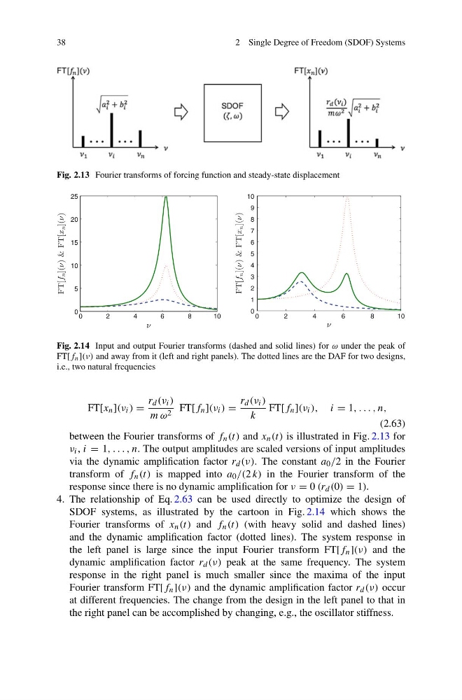
Fig. 2.13 Fourier transforms of forcing function and steady-state displacement
0
2
4
6
8
10
0
5
10
15
20
25
ν
FT[f
n ](ν) & FT[x
n ](ν)
0
2
4
6
8
10
0
1
2
3
4
5
6
7
8
9
10
ν
FT[f
n ](ν) & FT[x
n ](ν)
Fig. 2.14 Input and output Fourier transforms (dashed and solid lines) for ω under the peak of
FT[f n ](ν) and away from it (left and right panels). The dotted lines are the DAF for two designs,
i.e., two natural frequencies
FT[x n ](ν i ) =
r d (ν i )
m ω 2 FT[f n ](ν i ) =
r d (ν i )
k
FT[f n ](ν i ), i = 1, . . . , n,
(2.63)
between the Fourier transforms of f n (t) and x n (t) is illustrated in Fig. 2.13 for
ν i , i = 1, . . . , n. The output amplitudes are scaled versions of input amplitudes
via the dynamic amplification factor r d (ν). The constant a 0 /2 in the Fourier
transform of f n (t) is mapped into a 0 /(2 k) in the Fourier transform of the
response since there is no dynamic amplification for ν = 0 (r d (0) = 1).
4. The relationship of Eq. 2.63 can be used directly to optimize the design of
SDOF systems, as illustrated by the cartoon in Fig. 2.14 which shows the
Fourier transforms of x n (t) and f n (t) (with heavy solid and dashed lines)
and the dynamic amplification factor (dotted lines). The system response in
the left panel is large since the input Fourier transform FT[f n ](ν) and the
dynamic amplification factor r d (ν) peak at the same frequency. The system
response in the right panel is much smaller since the maxima of the input
Fourier transform FT[f n ](ν) and the dynamic amplification factor r d (ν) occur
at different frequencies. The change from the design in the left panel to that in
the right panel can be accomplished by changing, e.g., the oscillator stiffness.
2 Single Degree of Freedom (SDOF) Systems
Fig. 2.13 Fourier transforms of forcing function and steady-state displacement
0
2
4
6
8
10
0
5
10
15
20
25
ν
FT[f
n ](ν) & FT[x
n ](ν)
0
2
4
6
8
10
0
1
2
3
4
5
6
7
8
9
10
ν
FT[f
n ](ν) & FT[x
n ](ν)
Fig. 2.14 Input and output Fourier transforms (dashed and solid lines) for ω under the peak of
FT[f n ](ν) and away from it (left and right panels). The dotted lines are the DAF for two designs,
i.e., two natural frequencies
FT[x n ](ν i ) =
r d (ν i )
m ω 2 FT[f n ](ν i ) =
r d (ν i )
k
FT[f n ](ν i ), i = 1, . . . , n,
(2.63)
between the Fourier transforms of f n (t) and x n (t) is illustrated in Fig. 2.13 for
ν i , i = 1, . . . , n. The output amplitudes are scaled versions of input amplitudes
via the dynamic amplification factor r d (ν). The constant a 0 /2 in the Fourier
transform of f n (t) is mapped into a 0 /(2 k) in the Fourier transform of the
response since there is no dynamic amplification for ν = 0 (r d (0) = 1).
4. The relationship of Eq. 2.63 can be used directly to optimize the design of
SDOF systems, as illustrated by the cartoon in Fig. 2.14 which shows the
Fourier transforms of x n (t) and f n (t) (with heavy solid and dashed lines)
and the dynamic amplification factor (dotted lines). The system response in
the left panel is large since the input Fourier transform FT[f n ](ν) and the
dynamic amplification factor r d (ν) peak at the same frequency. The system
response in the right panel is much smaller since the maxima of the input
Fourier transform FT[f n ](ν) and the dynamic amplification factor r d (ν) occur
at different frequencies. The change from the design in the left panel to that in
the right panel can be accomplished by changing, e.g., the oscillator stiffness.