

2.6 Numerical Methods
39
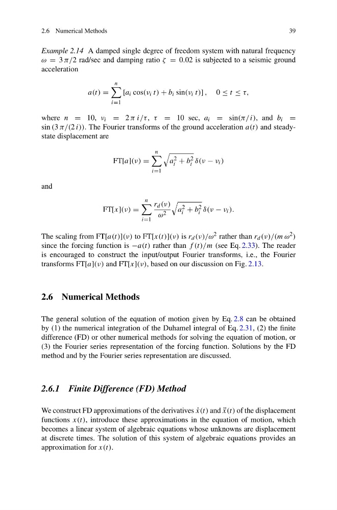
Example 2.14 A damped single degree of freedom system with natural frequency
ω = 3 π/2 rad/sec and damping ratio ζ = 0.02 is subjected to a seismic ground
acceleration
a(t) =
n
i=1
[a i cos(ν i t) + b i sin(ν i t)] , 0 ≤ t ≤ τ,
where n = 10, ν i = 2 π i/τ, τ = 10 sec, a i = sin(π/i), and b i =
sin (3 π/(2 i)). The Fourier transforms of the ground acceleration a(t) and steadystate displacement are
FT[a](ν) =
n
i=1
a 2
i + b 2
i δ(ν − ν i )
and
FT[x](ν) =
n
i=1
r d (ν)
ω 2
a 2
i + b 2
i δ(ν − ν i ).
The scaling from FT[a(t)](ν) to FT[x(t)](ν) is r d (ν)/ω 2 rather than r d (ν)/(m ω 2 )
since the forcing function is −a(t) rather than f (t)/m (see Eq. 2.33). The reader
is encouraged to construct the input/output Fourier transforms, i.e., the Fourier
transforms FT[a](ν) and FT[x](ν), based on our discussion on Fig. 2.13.
2.6 Numerical Methods
The general solution of the equation of motion given by Eq. 2.8 can be obtained
by (1) the numerical integration of the Duhamel integral of Eq. 2.31, (2) the finite
difference (FD) or other numerical methods for solving the equation of motion, or
(3) the Fourier series representation of the forcing function. Solutions by the FD
method and by the Fourier series representation are discussed.
2.6.1 Finite Difference (FD) Method
We construct FD approximations of the derivatives ˙
x(t) and ¨
x(t) of the displacement
functions x(t), introduce these approximations in the equation of motion, which
becomes a linear system of algebraic equations whose unknowns are displacement
at discrete times. The solution of this system of algebraic equations provides an
approximation for x(t).
39
Example 2.14 A damped single degree of freedom system with natural frequency
ω = 3 π/2 rad/sec and damping ratio ζ = 0.02 is subjected to a seismic ground
acceleration
a(t) =
n
i=1
[a i cos(ν i t) + b i sin(ν i t)] , 0 ≤ t ≤ τ,
where n = 10, ν i = 2 π i/τ, τ = 10 sec, a i = sin(π/i), and b i =
sin (3 π/(2 i)). The Fourier transforms of the ground acceleration a(t) and steadystate displacement are
FT[a](ν) =
n
i=1
a 2
i + b 2
i δ(ν − ν i )
and
FT[x](ν) =
n
i=1
r d (ν)
ω 2
a 2
i + b 2
i δ(ν − ν i ).
The scaling from FT[a(t)](ν) to FT[x(t)](ν) is r d (ν)/ω 2 rather than r d (ν)/(m ω 2 )
since the forcing function is −a(t) rather than f (t)/m (see Eq. 2.33). The reader
is encouraged to construct the input/output Fourier transforms, i.e., the Fourier
transforms FT[a](ν) and FT[x](ν), based on our discussion on Fig. 2.13.
2.6 Numerical Methods
The general solution of the equation of motion given by Eq. 2.8 can be obtained
by (1) the numerical integration of the Duhamel integral of Eq. 2.31, (2) the finite
difference (FD) or other numerical methods for solving the equation of motion, or
(3) the Fourier series representation of the forcing function. Solutions by the FD
method and by the Fourier series representation are discussed.
2.6.1 Finite Difference (FD) Method
We construct FD approximations of the derivatives ˙
x(t) and ¨
x(t) of the displacement
functions x(t), introduce these approximations in the equation of motion, which
becomes a linear system of algebraic equations whose unknowns are displacement
at discrete times. The solution of this system of algebraic equations provides an
approximation for x(t).