

5.1 Flexural Beams
121
similar to that of Eq. 5.12, which adds the components of the “vectors” ϕ r (x)
and ϕ n (x), i.e., the values of these functions at x ∈ [0, l]. The beam mass and
stiffness are not present in Eq. 5.12 since they do not depend on x.
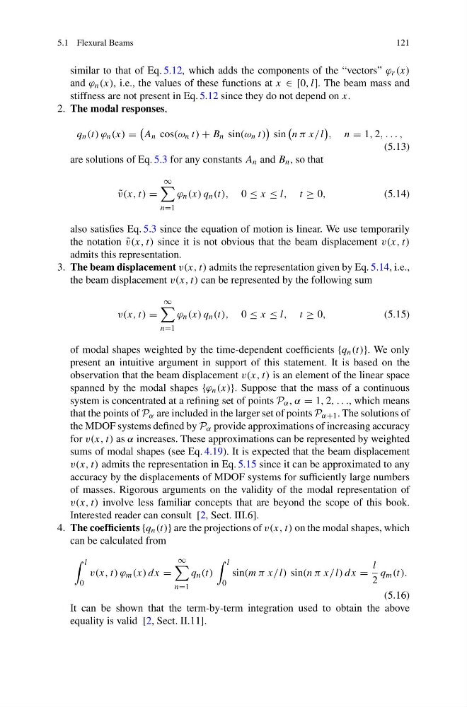
2. The modal responses,
q n (t) ϕ n (x) =
A n cos(ω n t) + B n sin(ω n t)
sin
n π x/l
, n = 1, 2, . . . ,
(5.13)
are solutions of Eq. 5.3 for any constants A n and B n , so that
˜
v(x, t) =
∞
n=1
ϕ n (x) q n (t), 0 ≤ x ≤ l, t ≥ 0,
(5.14)
also satisfies Eq. 5.3 since the equation of motion is linear. We use temporarily
the notation ˜
v(x, t) since it is not obvious that the beam displacement v(x, t)
admits this representation.
3. The beam displacement v(x, t) admits the representation given by Eq. 5.14, i.e.,
the beam displacement v(x, t) can be represented by the following sum
v(x, t) =
∞
n=1
ϕ n (x) q n (t), 0 ≤ x ≤ l, t ≥ 0,
(5.15)
of modal shapes weighted by the time-dependent coefficients {q n (t)}. We only
present an intuitive argument in support of this statement. It is based on the
observation that the beam displacement v(x, t) is an element of the linear space
spanned by the modal shapes {ϕ n (x)}. Suppose that the mass of a continuous
system is concentrated at a refining set of points P α , α = 1, 2, . . ., which means
that the points of P α are included in the larger set of points P α+1 . The solutions of
the MDOF systems defined by P α provide approximations of increasing accuracy
for v(x, t) as α increases. These approximations can be represented by weighted
sums of modal shapes (see Eq. 4.19). It is expected that the beam displacement
v(x, t) admits the representation in Eq. 5.15 since it can be approximated to any
accuracy by the displacements of MDOF systems for sufficiently large numbers
of masses. Rigorous arguments on the validity of the modal representation of
v(x, t) involve less familiar concepts that are beyond the scope of this book.
Interested reader can consult [2, Sect. III.6].
4. The coefficients {q n (t)} are the projections of v(x, t) on the modal shapes, which
can be calculated from
l
0
v(x, t) ϕ m (x) dx =
∞
n=1
q n (t)
l
0
sin(m π x/ l) sin(n π x/ l) dx =
l
2
q m (t).
(5.16)
It can be shown that the term-by-term integration used to obtain the above
equality is valid [2, Sect. II.11].
121
similar to that of Eq. 5.12, which adds the components of the “vectors” ϕ r (x)
and ϕ n (x), i.e., the values of these functions at x ∈ [0, l]. The beam mass and
stiffness are not present in Eq. 5.12 since they do not depend on x.
2. The modal responses,
q n (t) ϕ n (x) =
A n cos(ω n t) + B n sin(ω n t)
sin
n π x/l
, n = 1, 2, . . . ,
(5.13)
are solutions of Eq. 5.3 for any constants A n and B n , so that
˜
v(x, t) =
∞
n=1
ϕ n (x) q n (t), 0 ≤ x ≤ l, t ≥ 0,
(5.14)
also satisfies Eq. 5.3 since the equation of motion is linear. We use temporarily
the notation ˜
v(x, t) since it is not obvious that the beam displacement v(x, t)
admits this representation.
3. The beam displacement v(x, t) admits the representation given by Eq. 5.14, i.e.,
the beam displacement v(x, t) can be represented by the following sum
v(x, t) =
∞
n=1
ϕ n (x) q n (t), 0 ≤ x ≤ l, t ≥ 0,
(5.15)
of modal shapes weighted by the time-dependent coefficients {q n (t)}. We only
present an intuitive argument in support of this statement. It is based on the
observation that the beam displacement v(x, t) is an element of the linear space
spanned by the modal shapes {ϕ n (x)}. Suppose that the mass of a continuous
system is concentrated at a refining set of points P α , α = 1, 2, . . ., which means
that the points of P α are included in the larger set of points P α+1 . The solutions of
the MDOF systems defined by P α provide approximations of increasing accuracy
for v(x, t) as α increases. These approximations can be represented by weighted
sums of modal shapes (see Eq. 4.19). It is expected that the beam displacement
v(x, t) admits the representation in Eq. 5.15 since it can be approximated to any
accuracy by the displacements of MDOF systems for sufficiently large numbers
of masses. Rigorous arguments on the validity of the modal representation of
v(x, t) involve less familiar concepts that are beyond the scope of this book.
Interested reader can consult [2, Sect. III.6].
4. The coefficients {q n (t)} are the projections of v(x, t) on the modal shapes, which
can be calculated from
l
0
v(x, t) ϕ m (x) dx =
∞
n=1
q n (t)
l
0
sin(m π x/ l) sin(n π x/ l) dx =
l
2
q m (t).
(5.16)
It can be shown that the term-by-term integration used to obtain the above
equality is valid [2, Sect. II.11].