

120
5 Continuous Systems
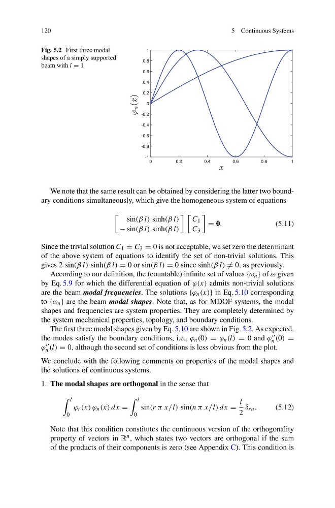
Fig. 5.2 First three modal
shapes of a simply supported
beam with l = 1
0
0.2
0.4
0.6
0.8
1
-1
-0.8
-0.6
-0.4
-0.2
0
0.2
0.4
0.6
0.8
1
We note that the same result can be obtained by considering the latter two boundary conditions simultaneously, which give the homogeneous system of equations
sin(β l) sinh(β l)
− sin(β l) sinh(β l)
C 1
C 3
= 0.
(5.11)
Since the trivial solution C 1 = C 3 = 0 is not acceptable, we set zero the determinant
of the above system of equations to identify the set of non-trivial solutions. This
gives 2 sin(β l) sinh(β l) = 0 or sin(β l) = 0 since sinh(β l) = 0, as previously.
According to our definition, the (countable) infinite set of values {ω n } of ω given
by Eq. 5.9 for which the differential equation of ϕ(x) admits non-trivial solutions
are the beam modal frequencies. The solutions {ϕ n (x)} in Eq. 5.10 corresponding
to {ω n } are the beam modal shapes. Note that, as for MDOF systems, the modal
shapes and frequencies are system properties. They are completely determined by
the system mechanical properties, topology, and boundary conditions.
The first three modal shapes given by Eq. 5.10 are shown in Fig. 5.2. As expected,
the modes satisfy the boundary conditions, i.e., ϕ n (0) = ϕ n (l) = 0 and ϕ
n (0) =
ϕ
n (l) = 0, although the second set of conditions is less obvious from the plot.
We conclude with the following comments on properties of the modal shapes and
the solutions of continuous systems.
1. The modal shapes are orthogonal in the sense that
l
0
ϕ r (x) ϕ n (x) dx =
l
0
sin(r π x/ l) sin(n π x/ l) dx =
l
2
δ rn .
(5.12)
Note that this condition constitutes the continuous version of the orthogonality
property of vectors in R n , which states two vectors are orthogonal if the sum
of the products of their components is zero (see Appendix C). This condition is
5 Continuous Systems
Fig. 5.2 First three modal
shapes of a simply supported
beam with l = 1
0
0.2
0.4
0.6
0.8
1
-1
-0.8
-0.6
-0.4
-0.2
0
0.2
0.4
0.6
0.8
1
We note that the same result can be obtained by considering the latter two boundary conditions simultaneously, which give the homogeneous system of equations
sin(β l) sinh(β l)
− sin(β l) sinh(β l)
C 1
C 3
= 0.
(5.11)
Since the trivial solution C 1 = C 3 = 0 is not acceptable, we set zero the determinant
of the above system of equations to identify the set of non-trivial solutions. This
gives 2 sin(β l) sinh(β l) = 0 or sin(β l) = 0 since sinh(β l) = 0, as previously.
According to our definition, the (countable) infinite set of values {ω n } of ω given
by Eq. 5.9 for which the differential equation of ϕ(x) admits non-trivial solutions
are the beam modal frequencies. The solutions {ϕ n (x)} in Eq. 5.10 corresponding
to {ω n } are the beam modal shapes. Note that, as for MDOF systems, the modal
shapes and frequencies are system properties. They are completely determined by
the system mechanical properties, topology, and boundary conditions.
The first three modal shapes given by Eq. 5.10 are shown in Fig. 5.2. As expected,
the modes satisfy the boundary conditions, i.e., ϕ n (0) = ϕ n (l) = 0 and ϕ
n (0) =
ϕ
n (l) = 0, although the second set of conditions is less obvious from the plot.
We conclude with the following comments on properties of the modal shapes and
the solutions of continuous systems.
1. The modal shapes are orthogonal in the sense that
l
0
ϕ r (x) ϕ n (x) dx =
l
0
sin(r π x/ l) sin(n π x/ l) dx =
l
2
δ rn .
(5.12)
Note that this condition constitutes the continuous version of the orthogonality
property of vectors in R n , which states two vectors are orthogonal if the sum
of the products of their components is zero (see Appendix C). This condition is