

5.1 Flexural Beams
119
The initial conditions and the selected values of ω are used to find the constants A
and B. The following example illustrates the construction of the modal shapes and
frequency for a simple continuous system.
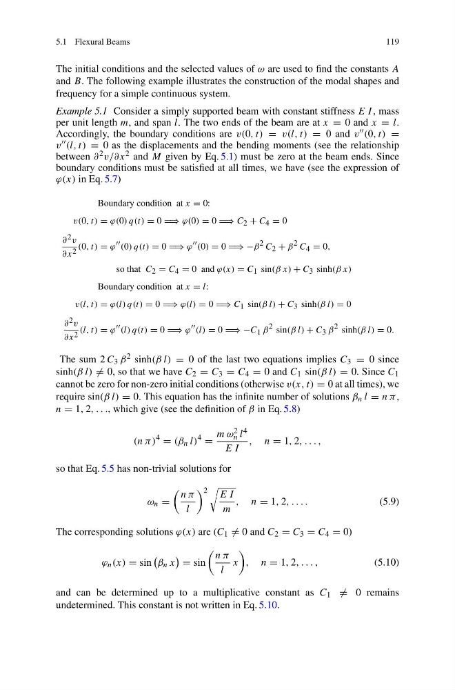
Example 5.1 Consider a simply supported beam with constant stiffness E I, mass
per unit length m, and span l. The two ends of the beam are at x = 0 and x = l.
Accordingly, the boundary conditions are v(0, t) = v(l, t) = 0 and v (0, t) =
v (l, t) = 0 as the displacements and the bending moments (see the relationship
between ∂ 2 v/∂x 2 and M given by Eq. 5.1) must be zero at the beam ends. Since
boundary conditions must be satisfied at all times, we have (see the expression of
ϕ(x) in Eq. 5.7)
Boundary condition at x = 0:
v(0, t) = ϕ(0) q(t) = 0 ⇒ ϕ(0) = 0 ⇒ C 2 + C 4 = 0
∂ 2 v
∂x 2 (0, t) = ϕ (0) q(t) = 0 ⇒ ϕ (0) = 0 ⇒ −β 2 C 2 + β 2 C 4 = 0,
so that C 2 = C 4 = 0 and ϕ(x) = C 1 sin(β x) + C 3 sinh(β x)
Boundary condition at x = l:
v(l, t) = ϕ(l) q(t) = 0 ⇒ ϕ(l) = 0 ⇒ C 1 sin(β l) + C 3 sinh(β l) = 0
∂ 2 v
∂x 2 (l, t) = ϕ (l) q(t) = 0 ⇒ ϕ (l) = 0 ⇒ −C 1 β 2 sin(β l) + C 3 β 2 sinh(β l) = 0.
The sum 2 C 3 β 2 sinh(β l) = 0 of the last two equations implies C 3 = 0 since
sinh(β l) = 0, so that we have C 2 = C 3 = C 4 = 0 and C 1 sin(β l) = 0. Since C 1
cannot be zero for non-zero initial conditions (otherwise v(x, t) = 0 at all times), we
require sin(β l) = 0. This equation has the infinite number of solutions β n l = n π,
n = 1, 2, . . ., which give (see the definition of β in Eq. 5.8)
(n π )
4
= (β n l)
4
=
m ω 2
n l 4
E I
, n = 1, 2, . . . ,
so that Eq. 5.5 has non-trivial solutions for
ω n =
n π
l
2
E I
m
, n = 1, 2, . . . .
(5.9)
The corresponding solutions ϕ(x) are (C 1 = 0 and C 2 = C 3 = C 4 = 0)
ϕ n (x) = sin
β n x
= sin
n π
l
x
, n = 1, 2, . . . ,
(5.10)
and can be determined up to a multiplicative constant as C 1 = 0 remains
undetermined. This constant is not written in Eq. 5.10.
119
The initial conditions and the selected values of ω are used to find the constants A
and B. The following example illustrates the construction of the modal shapes and
frequency for a simple continuous system.
Example 5.1 Consider a simply supported beam with constant stiffness E I, mass
per unit length m, and span l. The two ends of the beam are at x = 0 and x = l.
Accordingly, the boundary conditions are v(0, t) = v(l, t) = 0 and v (0, t) =
v (l, t) = 0 as the displacements and the bending moments (see the relationship
between ∂ 2 v/∂x 2 and M given by Eq. 5.1) must be zero at the beam ends. Since
boundary conditions must be satisfied at all times, we have (see the expression of
ϕ(x) in Eq. 5.7)
Boundary condition at x = 0:
v(0, t) = ϕ(0) q(t) = 0 ⇒ ϕ(0) = 0 ⇒ C 2 + C 4 = 0
∂ 2 v
∂x 2 (0, t) = ϕ (0) q(t) = 0 ⇒ ϕ (0) = 0 ⇒ −β 2 C 2 + β 2 C 4 = 0,
so that C 2 = C 4 = 0 and ϕ(x) = C 1 sin(β x) + C 3 sinh(β x)
Boundary condition at x = l:
v(l, t) = ϕ(l) q(t) = 0 ⇒ ϕ(l) = 0 ⇒ C 1 sin(β l) + C 3 sinh(β l) = 0
∂ 2 v
∂x 2 (l, t) = ϕ (l) q(t) = 0 ⇒ ϕ (l) = 0 ⇒ −C 1 β 2 sin(β l) + C 3 β 2 sinh(β l) = 0.
The sum 2 C 3 β 2 sinh(β l) = 0 of the last two equations implies C 3 = 0 since
sinh(β l) = 0, so that we have C 2 = C 3 = C 4 = 0 and C 1 sin(β l) = 0. Since C 1
cannot be zero for non-zero initial conditions (otherwise v(x, t) = 0 at all times), we
require sin(β l) = 0. This equation has the infinite number of solutions β n l = n π,
n = 1, 2, . . ., which give (see the definition of β in Eq. 5.8)
(n π )
4
= (β n l)
4
=
m ω 2
n l 4
E I
, n = 1, 2, . . . ,
so that Eq. 5.5 has non-trivial solutions for
ω n =
n π
l
2
E I
m
, n = 1, 2, . . . .
(5.9)
The corresponding solutions ϕ(x) are (C 1 = 0 and C 2 = C 3 = C 4 = 0)
ϕ n (x) = sin
β n x
= sin
n π
l
x
, n = 1, 2, . . . ,
(5.10)
and can be determined up to a multiplicative constant as C 1 = 0 remains
undetermined. This constant is not written in Eq. 5.10.