

106
4 Multi-Degree of Freedom (MDOF) Systems
u =
⎡
⎢
⎢
⎢
⎣
0.7812 + 0.0000 i 0.7812 + 0.0000 i 0.7543 + 0.0000 i 0.7543 + 0.0000 i
−0.5572 − 0.0097 i −0.5572 + 0.0097 i 0.3480 − 0.0730 i 0.3480 + 0.0730 i
0.0623 + 0.2215 i 0.0623 − 0.2215 i 0.1048 + 0.4891 i 0.1048 − 0.4891 i
−0.0297 − 0.1591 i −0.0297 + 0.1591 i 0.0580 + 0.2260 i 0.0580 − 0.2260 i
⎤
⎥
⎥
⎥
⎦
v =
⎡
⎢
⎢
⎢
⎣
−0.0169 − 0.1190 i −0.0169 + 0.1190 i −0.0591 − 0.3156 i −0.0591 + 0.3156 i
0.0579 + 0.2468 i 0.0579 − 0.2468 i −0.0649 − 0.4447 i −0.0649 + 0.4447 i
0.4094 + 0.0368 i 0.4094 − 0.0368 i 0.4843 − 0.0195 i 0.4843 + 0.0195 i
−0.8674 + 0.0000 i −0.8674 + 0.0000 i 0.6783 + 0.0000 i 0.6783 + 0.0000 i.
⎤
⎥
⎥
⎥
⎦
The modal coordinates {q i (t)} satisfy Eq. 4.88 with the forcing functions given by
the components
⎡
⎢
⎢
⎣
0.1629 + 0.0414 i
0.1629 − 0.0414 i
0.2083 + 0.0321 i
0.2083 − 0.0321 i
⎤
⎥
⎥
⎦ sin(t) kN.s/m
of the vector v T b f(t) scaled by the non-zero entries of the diagonal matrix v T u.
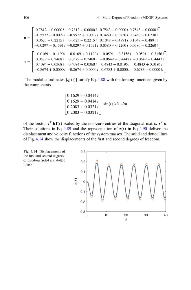
Their solutions in Eq. 4.89 and the representation of z(t) in Eq. 4.90 deliver the
displacement and velocity functions of the system masses. The solid and dotted lines
of Fig. 4.14 show the displacements of the first and second degrees of freedom.
Fig. 4.14 Displacements of
the first and second degrees
of freedom (solid and dotted
lines)
0
1 0
2 0
3 0
4 0
-0.3
-0.2
-0.1
0
0.1
0.2
0.3
4 Multi-Degree of Freedom (MDOF) Systems
u =
⎡
⎢
⎢
⎢
⎣
0.7812 + 0.0000 i 0.7812 + 0.0000 i 0.7543 + 0.0000 i 0.7543 + 0.0000 i
−0.5572 − 0.0097 i −0.5572 + 0.0097 i 0.3480 − 0.0730 i 0.3480 + 0.0730 i
0.0623 + 0.2215 i 0.0623 − 0.2215 i 0.1048 + 0.4891 i 0.1048 − 0.4891 i
−0.0297 − 0.1591 i −0.0297 + 0.1591 i 0.0580 + 0.2260 i 0.0580 − 0.2260 i
⎤
⎥
⎥
⎥
⎦
v =
⎡
⎢
⎢
⎢
⎣
−0.0169 − 0.1190 i −0.0169 + 0.1190 i −0.0591 − 0.3156 i −0.0591 + 0.3156 i
0.0579 + 0.2468 i 0.0579 − 0.2468 i −0.0649 − 0.4447 i −0.0649 + 0.4447 i
0.4094 + 0.0368 i 0.4094 − 0.0368 i 0.4843 − 0.0195 i 0.4843 + 0.0195 i
−0.8674 + 0.0000 i −0.8674 + 0.0000 i 0.6783 + 0.0000 i 0.6783 + 0.0000 i.
⎤
⎥
⎥
⎥
⎦
The modal coordinates {q i (t)} satisfy Eq. 4.88 with the forcing functions given by
the components
⎡
⎢
⎢
⎣
0.1629 + 0.0414 i
0.1629 − 0.0414 i
0.2083 + 0.0321 i
0.2083 − 0.0321 i
⎤
⎥
⎥
⎦ sin(t) kN.s/m
of the vector v T b f(t) scaled by the non-zero entries of the diagonal matrix v T u.
Their solutions in Eq. 4.89 and the representation of z(t) in Eq. 4.90 deliver the
displacement and velocity functions of the system masses. The solid and dotted lines
of Fig. 4.14 show the displacements of the first and second degrees of freedom.
Fig. 4.14 Displacements of
the first and second degrees
of freedom (solid and dotted
lines)
0
1 0
2 0
3 0
4 0
-0.3
-0.2
-0.1
0
0.1
0.2
0.3