

9 Towards the “Shape” of Cosmological Observables and the String …
225
in Fig. 9.4, we expect a long-lived 1-cycle, corresponding to the large “hole” in the
middle. Persistence allows us to assign a notion of significance to different topological features. This can be exploited to define distances between persistence diagrams
that enjoy nice stability properties.
In can be shown that when each p-simplex in a filtration is added to the simplicial complex, it either creates a p-cycle or destroys a ( p − 1)-cycle. In persistent
homology, we track individual topological features by computing the persistence
pair (σ, τ ) that create and destroy a particular homology class. The homology class
is then “born” when σ is added to the filtration and “dies” when τ is added. Given a
filtration containing N simplices, one can compute the persistence pairing in O(N
3
)
time, often quite faster, via linear algebra operations on the boundary operators [44].
9.2.3 Persistence Diagrams and Other Representations
One useful way to represent and interpret the result of of a persistent homology
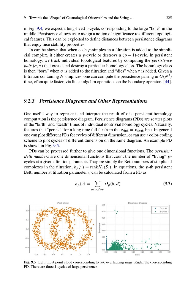
computation is the persistence diagram. Persistence diagrams (PDs) are scatter plots
of the “birth” and “death” times of individual nontrivial homology cycles. Naturally,
features that “persist” for a long time fall far from the ν birth = ν death line. In general
one can plot different PDs for cycles of different dimension, or can use a color-coding
scheme to plot cycles of different dimension on the same diagram. An example PD
is shown in Fig. 9.5.
PDs can be processed further to give one dimensional functions. The persistent
Betti numbers are one dimensional functions that count the number of “living” pcycles at a given filtration parameter. They are simply the Betti numbers of simplicial
complexes in the filtration, b p (ν) = rankH p (S ν ). In equations, the p-th persistent
Betti number at filtration parameter ν can be calculated from a PD as
b p (ν) =
b≤ν,d>ν
O p (b, d)
(9.3)
Fig. 9.5 Left: input point cloud corresponding to two overlapping rings. Right: the corresponding
PD. There are three 1-cycles of large persistence
225
in Fig. 9.4, we expect a long-lived 1-cycle, corresponding to the large “hole” in the
middle. Persistence allows us to assign a notion of significance to different topological features. This can be exploited to define distances between persistence diagrams
that enjoy nice stability properties.
In can be shown that when each p-simplex in a filtration is added to the simplicial complex, it either creates a p-cycle or destroys a ( p − 1)-cycle. In persistent
homology, we track individual topological features by computing the persistence
pair (σ, τ ) that create and destroy a particular homology class. The homology class
is then “born” when σ is added to the filtration and “dies” when τ is added. Given a
filtration containing N simplices, one can compute the persistence pairing in O(N
3
)
time, often quite faster, via linear algebra operations on the boundary operators [44].
9.2.3 Persistence Diagrams and Other Representations
One useful way to represent and interpret the result of of a persistent homology
computation is the persistence diagram. Persistence diagrams (PDs) are scatter plots
of the “birth” and “death” times of individual nontrivial homology cycles. Naturally,
features that “persist” for a long time fall far from the ν birth = ν death line. In general
one can plot different PDs for cycles of different dimension, or can use a color-coding
scheme to plot cycles of different dimension on the same diagram. An example PD
is shown in Fig. 9.5.
PDs can be processed further to give one dimensional functions. The persistent
Betti numbers are one dimensional functions that count the number of “living” pcycles at a given filtration parameter. They are simply the Betti numbers of simplicial
complexes in the filtration, b p (ν) = rankH p (S ν ). In equations, the p-th persistent
Betti number at filtration parameter ν can be calculated from a PD as
b p (ν) =
b≤ν,d>ν
O p (b, d)
(9.3)
Fig. 9.5 Left: input point cloud corresponding to two overlapping rings. Right: the corresponding
PD. There are three 1-cycles of large persistence