

30 Effect of a Hydrogen Sulfide-Containing Atmosphere on the Physical. . .
479
Fig. 30.4 Geometry of the
specimens tested and the
loading mode
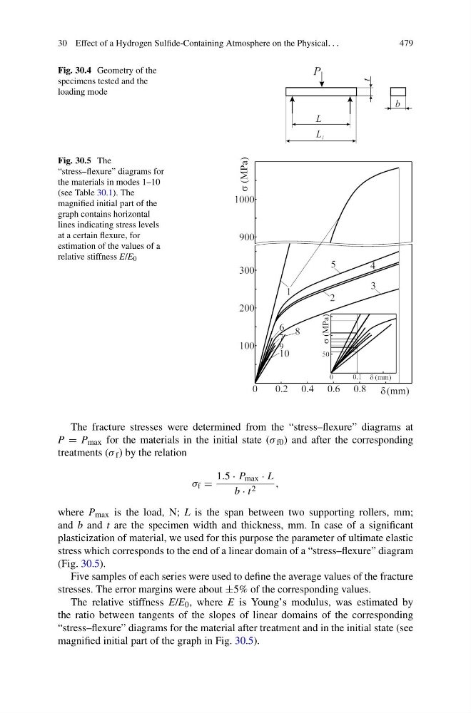
Fig. 30.5 The
“stress–flexure” diagrams for
the materials in modes 1–10
(see Table 30.1). The
magnified initial part of the
graph contains horizontal
lines indicating stress levels
at a certain flexure, for
estimation of the values of a
relative stiffness E/E 0
The fracture stresses were determined from the “stress–flexure” diagrams at
P = P max for the materials in the initial state (σ f0 ) and after the corresponding
treatments (σ f ) by the relation
σ f =
1.5 · P max · L
b · t 2
,
where P max is the load, N; L is the span between two supporting rollers, mm;
and b and t are the specimen width and thickness, mm. In case of a significant
plasticization of material, we used for this purpose the parameter of ultimate elastic
stress which corresponds to the end of a linear domain of a “stress–flexure” diagram
(Fig. 30.5).
Five samples of each series were used to define the average values of the fracture
stresses. The error margins were about ±5% of the corresponding values.
The relative stiffness E/E 0 , where E is Young’s modulus, was estimated by
the ratio between tangents of the slopes of linear domains of the corresponding
“stress–flexure” diagrams for the material after treatment and in the initial state (see
magnified initial part of the graph in Fig. 30.5).
479
Fig. 30.4 Geometry of the
specimens tested and the
loading mode
Fig. 30.5 The
“stress–flexure” diagrams for
the materials in modes 1–10
(see Table 30.1). The
magnified initial part of the
graph contains horizontal
lines indicating stress levels
at a certain flexure, for
estimation of the values of a
relative stiffness E/E 0
The fracture stresses were determined from the “stress–flexure” diagrams at
P = P max for the materials in the initial state (σ f0 ) and after the corresponding
treatments (σ f ) by the relation
σ f =
1.5 · P max · L
b · t 2
,
where P max is the load, N; L is the span between two supporting rollers, mm;
and b and t are the specimen width and thickness, mm. In case of a significant
plasticization of material, we used for this purpose the parameter of ultimate elastic
stress which corresponds to the end of a linear domain of a “stress–flexure” diagram
(Fig. 30.5).
Five samples of each series were used to define the average values of the fracture
stresses. The error margins were about ±5% of the corresponding values.
The relative stiffness E/E 0 , where E is Young’s modulus, was estimated by
the ratio between tangents of the slopes of linear domains of the corresponding
“stress–flexure” diagrams for the material after treatment and in the initial state (see
magnified initial part of the graph in Fig. 30.5).