

61
Human-Inspired Hyper Dynamic Manipulation
τ 2dv
τ 2da
β 21
β 21
I: +
II: +
III: −
IV: −
II: if 1 ≥ 0 –
¨
if 1 ≤ 0 +
¨
I: if 1 ≥ 0 +
¨
if 1 ≤ 0 –
¨
III: if 1 ≥ 0 –
¨
if 1 ≤ 0 +
¨
IV: if 1 ≥ 0 +
¨
if 1 ≤ 0 –
¨
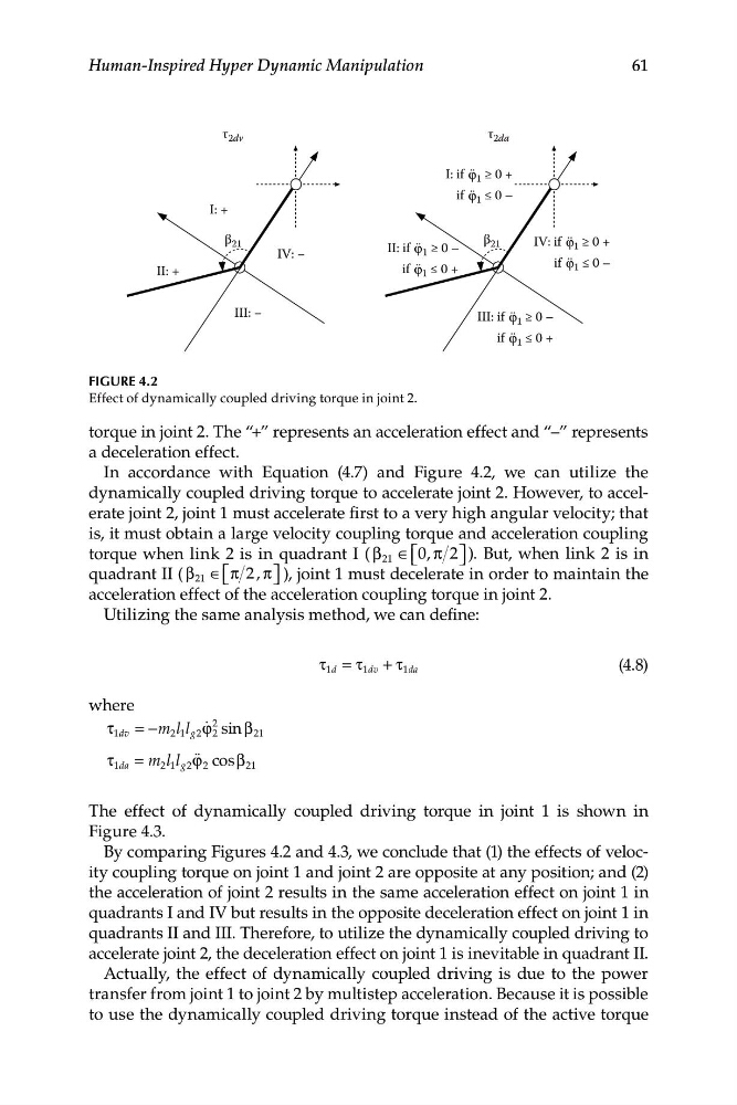
FIGURE 4.2
Effect of dynamically coupled driving torque in joint 2.
torque in joint 2. The “+” represents an acceleration effect and “–” represents
a deceleration effect.
In accordance with Equation (4.7) and Figure 4.2, we can utilize the
dynamically coupled driving torque to accelerate joint 2. However, to accelerate joint 2, joint 1 must accelerate first to a very high angular velocity; that
is, it must obtain a large velocity coupling torque and acceleration coupling
torque when link 2 is in quadrant I ( β 21 ∈⎡ ⎣ 0, π 2 ⎦ ⎤ ). But, when link 2 is in
quadrant II ( β 21 ∈⎡ ⎣ π 2 , π ⎦ ⎤ ), joint 1 must decelerate in order to maintain the
acceleration effect of the acceleration coupling torque in joint 2.
Utilizing the same analysis method, we can define:
τ d = τ d v + τ d a
(4 .8)
where
τ 1dv = −m l
2
2 1 l g 2 ϕ q 2 sin β 21
τ 1da = m l
21 l g 2 ϕ qq 2 cosβ 2 1
The effect of dynamically coupled driving torque in joint 1 is shown in
Figure 4.3.
By comparing Figures 4.2 and 4.3, we conclude that (1) the effects of velocity coupling torque on joint 1 and joint 2 are opposite at any position; and (2)
the acceleration of joint 2 results in the same acceleration effect on joint 1 in
quadrants I and IV but results in the opposite deceleration effect on joint 1 in
quadrants II and III. Therefore, to utilize the dynamically coupled driving to
accelerate joint 2, the deceleration effect on joint 1 is inevitable in quadrant II.
Actually, the effect of dynamically coupled driving is due to the power
transfer from joint 1 to joint 2 by multistep acceleration. Because it is possible
to use the dynamically coupled driving torque instead of the active torque
Human-Inspired Hyper Dynamic Manipulation
τ 2dv
τ 2da
β 21
β 21
I: +
II: +
III: −
IV: −
II: if 1 ≥ 0 –
¨
if 1 ≤ 0 +
¨
I: if 1 ≥ 0 +
¨
if 1 ≤ 0 –
¨
III: if 1 ≥ 0 –
¨
if 1 ≤ 0 +
¨
IV: if 1 ≥ 0 +
¨
if 1 ≤ 0 –
¨
FIGURE 4.2
Effect of dynamically coupled driving torque in joint 2.
torque in joint 2. The “+” represents an acceleration effect and “–” represents
a deceleration effect.
In accordance with Equation (4.7) and Figure 4.2, we can utilize the
dynamically coupled driving torque to accelerate joint 2. However, to accelerate joint 2, joint 1 must accelerate first to a very high angular velocity; that
is, it must obtain a large velocity coupling torque and acceleration coupling
torque when link 2 is in quadrant I ( β 21 ∈⎡ ⎣ 0, π 2 ⎦ ⎤ ). But, when link 2 is in
quadrant II ( β 21 ∈⎡ ⎣ π 2 , π ⎦ ⎤ ), joint 1 must decelerate in order to maintain the
acceleration effect of the acceleration coupling torque in joint 2.
Utilizing the same analysis method, we can define:
τ d = τ d v + τ d a
(4 .8)
where
τ 1dv = −m l
2
2 1 l g 2 ϕ q 2 sin β 21
τ 1da = m l
21 l g 2 ϕ qq 2 cosβ 2 1
The effect of dynamically coupled driving torque in joint 1 is shown in
Figure 4.3.
By comparing Figures 4.2 and 4.3, we conclude that (1) the effects of velocity coupling torque on joint 1 and joint 2 are opposite at any position; and (2)
the acceleration of joint 2 results in the same acceleration effect on joint 1 in
quadrants I and IV but results in the opposite deceleration effect on joint 1 in
quadrants II and III. Therefore, to utilize the dynamically coupled driving to
accelerate joint 2, the deceleration effect on joint 1 is inevitable in quadrant II.
Actually, the effect of dynamically coupled driving is due to the power
transfer from joint 1 to joint 2 by multistep acceleration. Because it is possible
to use the dynamically coupled driving torque instead of the active torque