60
Biologically Inspired Robotics
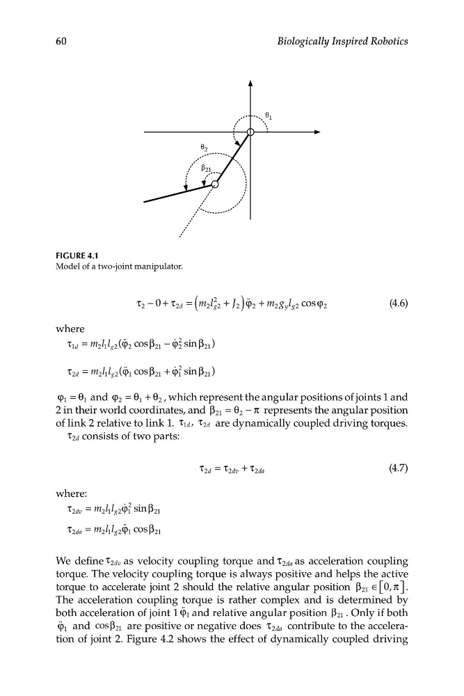
θ 1
θ 2
β 21
FIGURE 4.1
Model of a two-joint manipulator.
τ 0 τ = m l
2
+ J ϕ + m g l cos ϕ
(4.6)
− +
qq
2
2d
( 2 g2 2 ) 2 2 yg 2 2
where
τ = m l l (ϕ qq cos β − ϕ q 2 sin β )
1d
21 g 2
2
2 1
2
21
τ = m l l ϕ qq
β + ϕ
2
( cos
q sin β )
2d
21 g2
1
2 1
1
21
and ϕ θ θ
= 1
2 in their world coordinates, and β 21 θ π
− represents the angular position
ϕ θ
=
2
+ 2 , which represent the angular positions of joints 1 and
= 2
1
G
of link 2 relative to link 1. τ τ
G , 2 are dynamically coupled driving torques.
τ G consists of two parts:
τ d = τ d v + τ d a
(4.7)
where:
τ = m l l ϕ q 2 sin β
2dv
21 g2 1
21
= m l l qq
τ 2da
21 g2 ϕ 1 cosβ 2 1
We define τ dv as velocity coupling torque and τ da as acceleration coupling
torque. The velocity coupling torque is always positive and helps the active
torque to accelerate joint 2 should the relative angular position β 21 ∈ ⎣ ⎡0, π ⎦ ⎤ .
The acceleration coupling torque is rather complex and is determined by
both acceleration of joint 1 ϕ qq and relative angular position β 21 . Only if both
ϕ qq and cosβ 21 are positive or negative does τ da contribute to the acceleration of joint 2. Figure  4.2 shows the effect of dynamically coupled driving