

253
Multifunctional Actuators for Assistive Knee Braces
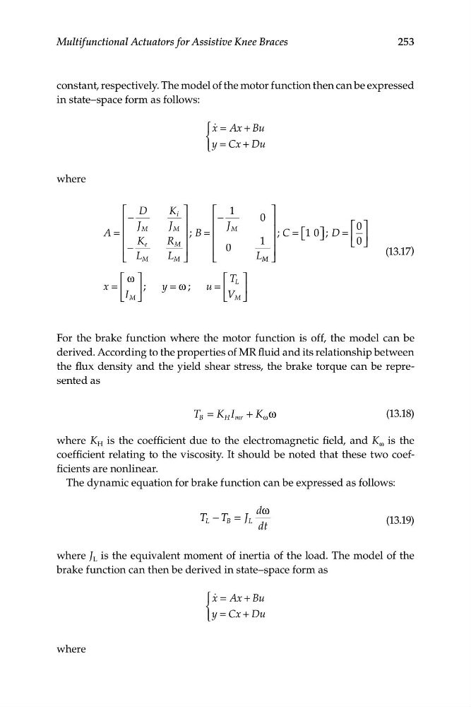
constant, respectively. The model of the motor function then can be expressed
in state–space form as follows:
⎧ x A
q = x + Bu
⎨
⎩ ⎪ y C
= x +
Du
where
⎡
D
K
−
i ⎤
⎡
1
⎤
⎢
⎥
⎢
−
0
⎥
J M
J
M
J
M
⎡
0
⎤
A
=
⎢
⎥ ;
B
=
⎢
⎥ ;
C
= ⎡ ⎣ 1 0 ⎦ ⎤ ;
D
= ⎢ ⎥
⎢ K
−
e
R
M
⎥
⎢
1
⎥
⎣ 0
⎦
⎢
⎥
⎢ 0
⎥
(13.17)
⎣
L M
L
M
⎦
⎣
L
M M ⎦
⎡ ω ⎤
⎡ T L ⎤
x
=
⎢ ⎥ ;
y
=
ω
;
u
=
⎢ ⎥
⎣ ⎣
I M ⎦
⎣ V M ⎦
For the brake function where the motor function is off, the model can be
derived. According to the properties of MR fluid and its relationship between
the flux density and the yield shear stress, the brake torque can be represented as
T B = K H I
mr +
K
ω ω
(13.18)
where K H is the coefficient due to the electromagnetic field, and K ω is the
coefficient relating to the viscosity. It should be noted that these two coefficients are nonlinear.
The dynamic equation for brake function can be expressed as follows:
dω
T L − T B = J L
(13.19)
dt
where J L is the equivalent moment of inertia of the load. The model of the
brake function can then be derived in state–space form as
⎧ x A
q = x + Bu
⎨
⎪ ⎩
+
y C
= x Du
where
Multifunctional Actuators for Assistive Knee Braces
constant, respectively. The model of the motor function then can be expressed
in state–space form as follows:
⎧ x A
q = x + Bu
⎨
⎩ ⎪ y C
= x +
Du
where
⎡
D
K
−
i ⎤
⎡
1
⎤
⎢
⎥
⎢
−
0
⎥
J M
J
M
J
M
⎡
0
⎤
A
=
⎢
⎥ ;
B
=
⎢
⎥ ;
C
= ⎡ ⎣ 1 0 ⎦ ⎤ ;
D
= ⎢ ⎥
⎢ K
−
e
R
M
⎥
⎢
1
⎥
⎣ 0
⎦
⎢
⎥
⎢ 0
⎥
(13.17)
⎣
L M
L
M
⎦
⎣
L
M M ⎦
⎡ ω ⎤
⎡ T L ⎤
x
=
⎢ ⎥ ;
y
=
ω
;
u
=
⎢ ⎥
⎣ ⎣
I M ⎦
⎣ V M ⎦
For the brake function where the motor function is off, the model can be
derived. According to the properties of MR fluid and its relationship between
the flux density and the yield shear stress, the brake torque can be represented as
T B = K H I
mr +
K
ω ω
(13.18)
where K H is the coefficient due to the electromagnetic field, and K ω is the
coefficient relating to the viscosity. It should be noted that these two coefficients are nonlinear.
The dynamic equation for brake function can be expressed as follows:
dω
T L − T B = J L
(13.19)
dt
where J L is the equivalent moment of inertia of the load. The model of the
brake function can then be derived in state–space form as
⎧ x A
q = x + Bu
⎨
⎪ ⎩
+
y C
= x Du
where