

232
Biologically Inspired Robotics
⎛
^
M t
n ( ) ∑
u
=
b
⎜ f
n
⎞
P t f
, ⎟
f l
= b ⎝
( ) ⎠
(12.18)
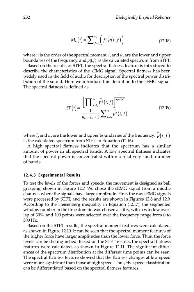
where n is the order of the spectral moment, l b and u b are the lower and upper
boundaries of the frequency, and p(t,f) is the calculated spectrum from STFT.
Based on the results of STFT, the spectral flatness feature is introduced to
describe the characteristics of the sEMG signal. Spectral flatness has been
widely used in the field of audio for description of the spectral power distribution of the sound. Here we introduce this definition to the sEMG signal.
The spectral flatness is defined as
1
⎡
u b
^
u l
b − +
b 1
⎢∏
P
2 t f
=
(
( )
⎣
=
f l b
)
⎤
, ⎥ ⎦
SF t
(12.19
1
∑
)
u b
^ ^
P
2
(t f
, )
u b − +
l 1
f l
=
b
b
^
where l b and u b are the lower and upper boundaries of the frequency. P( t f
, )
is the calculated spectrum from STFT in Equation (12.16).
A high spectral flatness indicates that the spectrum has a similar
amount of power in all spectral bands. A low spectral flatness indicates
that the spectral power is concentrated within a relatively small number
of bands.
12.4.3 Experimental Results
To test the levels of the forces and speeds, the movement is designed as ball
grasping, shown in Figure 12.7. We chose the sEMG signal from a middle
channel, where the signals have large amplitude. First, the raw sEMG signals
were processed by STFT, and the results are shown in Figures 12.8 and 12.9.
According to the Heisenberg inequality in Equation (12.17), the segmented
window number in the time domain was chosen as fifty, with a window overlap of 30%, and 100 points were selected over the frequency range from 0 to
500 Hz.
Based on the STFT results, the spectral moment features were calculated,
as shown in Figure 12.10. It can be seen that the spectral moment features of
the higher force have larger amplitudes than the lower force. Thus, the force
levels can be distinguished. Based on the STFT results, the spectral flatness
features were calculated, as shown in Figure 12.11. The significant differences of the spectrum distribution at the different time points can be seen.
The spectral flatness feature showed that the flatness changes at low speed
were more significant than those at high speed. Thus, the speed classification
can be differentiated based on the spectral flatness features.
Biologically Inspired Robotics
⎛
^
M t
n ( ) ∑
u
=
b
⎜ f
n
⎞
P t f
, ⎟
f l
= b ⎝
( ) ⎠
(12.18)
where n is the order of the spectral moment, l b and u b are the lower and upper
boundaries of the frequency, and p(t,f) is the calculated spectrum from STFT.
Based on the results of STFT, the spectral flatness feature is introduced to
describe the characteristics of the sEMG signal. Spectral flatness has been
widely used in the field of audio for description of the spectral power distribution of the sound. Here we introduce this definition to the sEMG signal.
The spectral flatness is defined as
1
⎡
u b
^
u l
b − +
b 1
⎢∏
P
2 t f
=
(
( )
⎣
=
f l b
)
⎤
, ⎥ ⎦
SF t
(12.19
1
∑
)
u b
^ ^
P
2
(t f
, )
u b − +
l 1
f l
=
b
b
^
where l b and u b are the lower and upper boundaries of the frequency. P( t f
, )
is the calculated spectrum from STFT in Equation (12.16).
A high spectral flatness indicates that the spectrum has a similar
amount of power in all spectral bands. A low spectral flatness indicates
that the spectral power is concentrated within a relatively small number
of bands.
12.4.3 Experimental Results
To test the levels of the forces and speeds, the movement is designed as ball
grasping, shown in Figure 12.7. We chose the sEMG signal from a middle
channel, where the signals have large amplitude. First, the raw sEMG signals
were processed by STFT, and the results are shown in Figures 12.8 and 12.9.
According to the Heisenberg inequality in Equation (12.17), the segmented
window number in the time domain was chosen as fifty, with a window overlap of 30%, and 100 points were selected over the frequency range from 0 to
500 Hz.
Based on the STFT results, the spectral moment features were calculated,
as shown in Figure 12.10. It can be seen that the spectral moment features of
the higher force have larger amplitudes than the lower force. Thus, the force
levels can be distinguished. Based on the STFT results, the spectral flatness
features were calculated, as shown in Figure 12.11. The significant differences of the spectrum distribution at the different time points can be seen.
The spectral flatness feature showed that the flatness changes at low speed
were more significant than those at high speed. Thus, the speed classification
can be differentiated based on the spectral flatness features.