

170
Biologically Inspired Robotics
Y
X
F
L
h
δ
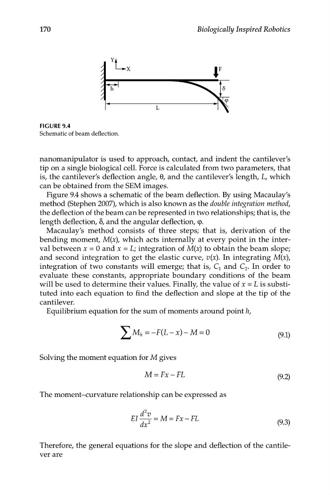
FIGURE 9.4
Schematic of beam deflection.
nanomanipulator is used to approach, contact, and indent the cantilever’s
tip on a single biological cell. Force is calculated from two parameters, that
is, the cantilever’s deflection angle, θ, and the cantilever’s length, L, which
can be obtained from the SEM images.
Figure 9.4 shows a schematic of the beam deflection. By using Macaulay’s
method (Stephen 2007), which is also known as the double integration method,
the deflection of the beam can be represented in two relationships; that is, the
length deflection, δ, and the angular deflection, φ.
Macaulay’s method consists of three steps; that is, derivation of the
bending moment, M(x), which acts internally at every point in the interval between x = 0 and x = L; integration of M(x) to obtain the beam slope;
and second integration to get the elastic curve, v(x). In integrating M(x),
integration of two constants will emerge; that is, C 1 and C 2 . In order to
evaluate these constants, appropriate boundary conditions of the beam
will be used to determine their values. Finally, the value of x = L is substituted into each equation to find the deflection and slope at the tip of the
cantilever.
Equilibrium equation for the sum of moments around point h,
∑ M h = −F L − x) − M
(9.1)
(
= 0
Solving the moment equation for M gives
M Fx − L
=
F
(9.2)
The moment–curvature relationship can be expressed as
d v
EI
= M F − FL
dx
= x
(9.3)
Therefore, the general equations for the slope and deflection of the cantilever are
Biologically Inspired Robotics
Y
X
F
L
h
δ
FIGURE 9.4
Schematic of beam deflection.
nanomanipulator is used to approach, contact, and indent the cantilever’s
tip on a single biological cell. Force is calculated from two parameters, that
is, the cantilever’s deflection angle, θ, and the cantilever’s length, L, which
can be obtained from the SEM images.
Figure 9.4 shows a schematic of the beam deflection. By using Macaulay’s
method (Stephen 2007), which is also known as the double integration method,
the deflection of the beam can be represented in two relationships; that is, the
length deflection, δ, and the angular deflection, φ.
Macaulay’s method consists of three steps; that is, derivation of the
bending moment, M(x), which acts internally at every point in the interval between x = 0 and x = L; integration of M(x) to obtain the beam slope;
and second integration to get the elastic curve, v(x). In integrating M(x),
integration of two constants will emerge; that is, C 1 and C 2 . In order to
evaluate these constants, appropriate boundary conditions of the beam
will be used to determine their values. Finally, the value of x = L is substituted into each equation to find the deflection and slope at the tip of the
cantilever.
Equilibrium equation for the sum of moments around point h,
∑ M h = −F L − x) − M
(9.1)
(
= 0
Solving the moment equation for M gives
M Fx − L
=
F
(9.2)
The moment–curvature relationship can be expressed as
d v
EI
= M F − FL
dx
= x
(9.3)
Therefore, the general equations for the slope and deflection of the cantilever are