

118
W. Annayat and B. S. Sil
3.2 Time Sequence Maps
Scanning of Landsat images is done and then imported in Arc GIS format. For
radiometric corrections, haze corrections and filtration of images ERDAS 9.1 were
used. From the processed images, the area of interest was extracted. Eye interpretation
and digital image processing techniques are used to delineate the bank lines, and then,
the delineated bank lines are used to generate a channel centreline with the help of
onscreen digitization in Arc Map.
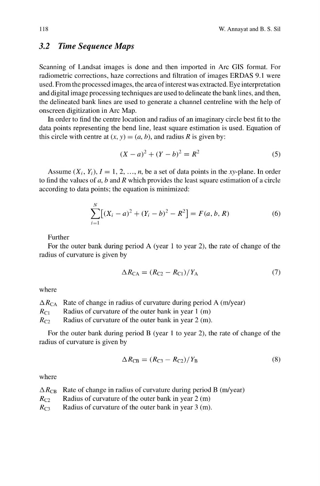
In order to find the centre location and radius of an imaginary circle best fit to the
data points representing the bend line, least square estimation is used. Equation of
this circle with centre at (x, y) = (a, b), and radius R is given by:
(X − a)
2
+ (Y − b)
2
= R
2
(5)
Assume (X i , Y i ), I = 1, 2, …, n, be a set of data points in the xy-plane. In order
to find the values of a, b and R which provides the least square estimation of a circle
according to data points; the equation is minimized:
N
i=1
(X i − a)
2
+ (Y i − b)
2
− R
2
= F(a, b, R)
(6)
Further
For the outer bank during period A (year 1 to year 2), the rate of change of the
radius of curvature is given by
R CA = (R C2 − R C1 )/Y A
(7)
where
R CA Rate of change in radius of curvature during period A (m/year)
R C1
Radius of curvature of the outer bank in year 1 (m)
R C2
Radius of curvature of the outer bank in year 2 (m).
For the outer bank during period B (year 1 to year 2), the rate of change of the
radius of curvature is given by
R CB = (R C3 − R C2 )/Y B
(8)
where
R CB Rate of change in radius of curvature during period B (m/year)
R C2
Radius of curvature of the outer bank in year 2 (m)
R C3
Radius of curvature of the outer bank in year 3 (m).
W. Annayat and B. S. Sil
3.2 Time Sequence Maps
Scanning of Landsat images is done and then imported in Arc GIS format. For
radiometric corrections, haze corrections and filtration of images ERDAS 9.1 were
used. From the processed images, the area of interest was extracted. Eye interpretation
and digital image processing techniques are used to delineate the bank lines, and then,
the delineated bank lines are used to generate a channel centreline with the help of
onscreen digitization in Arc Map.
In order to find the centre location and radius of an imaginary circle best fit to the
data points representing the bend line, least square estimation is used. Equation of
this circle with centre at (x, y) = (a, b), and radius R is given by:
(X − a)
2
+ (Y − b)
2
= R
2
(5)
Assume (X i , Y i ), I = 1, 2, …, n, be a set of data points in the xy-plane. In order
to find the values of a, b and R which provides the least square estimation of a circle
according to data points; the equation is minimized:
N
i=1
(X i − a)
2
+ (Y i − b)
2
− R
2
= F(a, b, R)
(6)
Further
For the outer bank during period A (year 1 to year 2), the rate of change of the
radius of curvature is given by
R CA = (R C2 − R C1 )/Y A
(7)
where
R CA Rate of change in radius of curvature during period A (m/year)
R C1
Radius of curvature of the outer bank in year 1 (m)
R C2
Radius of curvature of the outer bank in year 2 (m).
For the outer bank during period B (year 1 to year 2), the rate of change of the
radius of curvature is given by
R CB = (R C3 − R C2 )/Y B
(8)
where
R CB Rate of change in radius of curvature during period B (m/year)
R C2
Radius of curvature of the outer bank in year 2 (m)
R C3
Radius of curvature of the outer bank in year 3 (m).