

A Few Simple Models
Milankovitch’s accomplishment was to calculate the orbital
parameters of the Earth and the associated insolation
occurring over hundreds of thousands of years. Neither a
model of evolution of the ice caps nor a climate model was
available at this time. He simply linked the minimums in the
astronomical forcing with episodes of glaciation. He
explained that due to a very high probably inertia in the caps,
there would be a gap of several thousand years between the
astronomical forcing and the evolution of the caps, even to
the point of ‘smoothing’ the astronomical forcing if the caps
do not have the time to react. Indeed, the volume of the caps
is not directly related to the insolation, but rather it is the
variation in the volume of ice which is a function of insolation. In other words, an extremely simple model of evolution of the caps consists of integrating the astronomical
forcing over time. As the important physical object is the
cap, it is essential to look at the dynamics of the cap, not
only the forcing.
Surprisingly, no scientist seems to have focused on this
task, following either in the footsteps of Adhémar or Croll,
or those of Milankovitch. It was therefore a journalist
(Calder 1974) who would publish a scientific article
describing, for the first time, a model of ice cap evolution in
the Quaternary, more than a century after the ice ages were
observed. This model was both very simple and informative.
It is based on a simple integration of the forcing [see Paillard
(2001, 2010, 2015)]:
dV=dt ¼ Àkði À i 0 Þ:
where V is the volume of the cap and i(t) is the astronomical
forcing, i.e. summer insolation at the high latitudes of the
northern hemisphere. Above a fixed isolation value i 0 , the
volume of ice V decreases proportionally to i-i 0 and, below
this value, V increases. This model works relatively well
provided that an asymmetry between the melting and
accumulation episodes is introduced, with a different k coefficient in the two cases, k = k F and k A depending on
whether i > i 0 (melting) or not. In addition, V is imposed as a
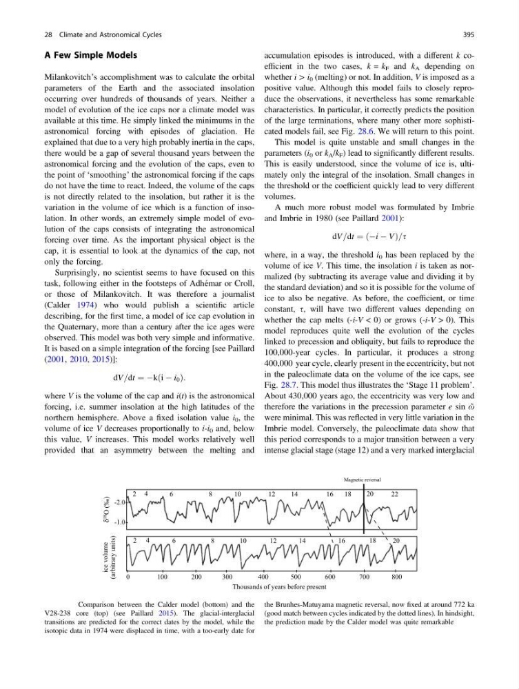
positive value. Although this model fails to closely reproduce the observations, it nevertheless has some remarkable
characteristics. In particular, it correctly predicts the position
of the large terminations, where many other more sophisticated models fail, see Fig. 28.6. We will return to this point.
This model is quite unstable and small changes in the
parameters (i 0 or k A /k F ) lead to significantly different results.
This is easily understood, since the volume of ice is, ultimately only the integral of the insolation. Small changes in
the threshold or the coefficient quickly lead to very different
volumes.
A much more robust model was formulated by Imbrie
and Imbrie in 1980 (see Paillard 2001):
dV=dt ¼ ðÀi À VÞ=s
where, in a way, the threshold i 0 has been replaced by the
volume of ice V. This time, the insolation i is taken as normalized (by subtracting its average value and dividing it by
the standard deviation) and so it is possible for the volume of
ice to also be negative. As before, the coefficient, or time
constant, s, will have two different values depending on
whether the cap melts (-i-V < 0) or grows (-i-V > 0). This
model reproduces quite well the evolution of the cycles
linked to precession and obliquity, but fails to reproduce the
100,000-year cycles. In particular, it produces a strong
400,000 year cycle, clearly present in the eccentricity, but not
in the paleoclimate data on the volume of the ice caps, see
Fig. 28.7. This model thus illustrates the ‘Stage 11 problem’.
About 430,000 years ago, the eccentricity was very low and
therefore the variations in the precession parameter e sin ῶ
were minimal. This was reflected in very little variation in the
Imbrie model. Conversely, the paleoclimate data show that
this period corresponds to a major transition between a very
intense glacial stage (stage 12) and a very marked interglacial
Magnetic reversal
2 4
6
8
0
1
1 2
1 4
1 6
1 8
20
22
2 4
6
1 0
8
1 2
1 4
1 6
18
20
0
100
200
300
400
500
600
700
800
Thousands of years before present
(arbitrary units)
δ
18
O (‰)
-2.0
-1.0
ice volume
Fig. 28.6 Comparison between the Calder model (bottom) and the
V28-238 core (top) (see Paillard 2015). The glacial-interglacial
transitions are predicted for the correct dates by the model, while the
isotopic data in 1974 were displaced in time, with a too-early date for
the Brunhes-Matuyama magnetic reversal, now fixed at around 772 ka
(good match between cycles indicated by the dotted lines). In hindsight,
the prediction made by the Calder model was quite remarkable
28 Climate and Astronomical Cycles
395
Milankovitch’s accomplishment was to calculate the orbital
parameters of the Earth and the associated insolation
occurring over hundreds of thousands of years. Neither a
model of evolution of the ice caps nor a climate model was
available at this time. He simply linked the minimums in the
astronomical forcing with episodes of glaciation. He
explained that due to a very high probably inertia in the caps,
there would be a gap of several thousand years between the
astronomical forcing and the evolution of the caps, even to
the point of ‘smoothing’ the astronomical forcing if the caps
do not have the time to react. Indeed, the volume of the caps
is not directly related to the insolation, but rather it is the
variation in the volume of ice which is a function of insolation. In other words, an extremely simple model of evolution of the caps consists of integrating the astronomical
forcing over time. As the important physical object is the
cap, it is essential to look at the dynamics of the cap, not
only the forcing.
Surprisingly, no scientist seems to have focused on this
task, following either in the footsteps of Adhémar or Croll,
or those of Milankovitch. It was therefore a journalist
(Calder 1974) who would publish a scientific article
describing, for the first time, a model of ice cap evolution in
the Quaternary, more than a century after the ice ages were
observed. This model was both very simple and informative.
It is based on a simple integration of the forcing [see Paillard
(2001, 2010, 2015)]:
dV=dt ¼ Àkði À i 0 Þ:
where V is the volume of the cap and i(t) is the astronomical
forcing, i.e. summer insolation at the high latitudes of the
northern hemisphere. Above a fixed isolation value i 0 , the
volume of ice V decreases proportionally to i-i 0 and, below
this value, V increases. This model works relatively well
provided that an asymmetry between the melting and
accumulation episodes is introduced, with a different k coefficient in the two cases, k = k F and k A depending on
whether i > i 0 (melting) or not. In addition, V is imposed as a
positive value. Although this model fails to closely reproduce the observations, it nevertheless has some remarkable
characteristics. In particular, it correctly predicts the position
of the large terminations, where many other more sophisticated models fail, see Fig. 28.6. We will return to this point.
This model is quite unstable and small changes in the
parameters (i 0 or k A /k F ) lead to significantly different results.
This is easily understood, since the volume of ice is, ultimately only the integral of the insolation. Small changes in
the threshold or the coefficient quickly lead to very different
volumes.
A much more robust model was formulated by Imbrie
and Imbrie in 1980 (see Paillard 2001):
dV=dt ¼ ðÀi À VÞ=s
where, in a way, the threshold i 0 has been replaced by the
volume of ice V. This time, the insolation i is taken as normalized (by subtracting its average value and dividing it by
the standard deviation) and so it is possible for the volume of
ice to also be negative. As before, the coefficient, or time
constant, s, will have two different values depending on
whether the cap melts (-i-V < 0) or grows (-i-V > 0). This
model reproduces quite well the evolution of the cycles
linked to precession and obliquity, but fails to reproduce the
100,000-year cycles. In particular, it produces a strong
400,000 year cycle, clearly present in the eccentricity, but not
in the paleoclimate data on the volume of the ice caps, see
Fig. 28.7. This model thus illustrates the ‘Stage 11 problem’.
About 430,000 years ago, the eccentricity was very low and
therefore the variations in the precession parameter e sin ῶ
were minimal. This was reflected in very little variation in the
Imbrie model. Conversely, the paleoclimate data show that
this period corresponds to a major transition between a very
intense glacial stage (stage 12) and a very marked interglacial
Magnetic reversal
2 4
6
8
0
1
1 2
1 4
1 6
1 8
20
22
2 4
6
1 0
8
1 2
1 4
1 6
18
20
0
100
200
300
400
500
600
700
800
Thousands of years before present
(arbitrary units)
δ
18
O (‰)
-2.0
-1.0
ice volume
Fig. 28.6 Comparison between the Calder model (bottom) and the
V28-238 core (top) (see Paillard 2015). The glacial-interglacial
transitions are predicted for the correct dates by the model, while the
isotopic data in 1974 were displaced in time, with a too-early date for
the Brunhes-Matuyama magnetic reversal, now fixed at around 772 ka
(good match between cycles indicated by the dotted lines). In hindsight,
the prediction made by the Calder model was quite remarkable
28 Climate and Astronomical Cycles
395