

to date past recordings. Indeed, a persistent difficulty in
paleoclimate reconstructions is the establishment of a reliable chronology. As such, absolute dating obtained from the
radioactive decay of certain isotopes (
14 C,
40 K/
39 Ar,
40 Ar/
39 Ar, U/Th) is often rare and difficult to obtain.
Moreover, they are imprecise. For example, a 1% error in the
measured age translates to an error of 10,000 years for
samples of one million years. The error only grows as one
goes back in time. It is therefore extremely tempting to use
astronomical theory to identify the cycles measured in a
paleoclimate recording by referring to the cycles of the
astronomical forcing. This link seems particularly relevant
for precession or obliquity, at least for the Quaternary. In the
case where correct identification of all the cycles is possible,
which turns out to be quite frequently, this methodology has
the enormous advantage of having an associated error which
does not increase disproportionately with time. This is
because if one does not ‘skip’ a cycle, then only the phase
relationship between the forcing and climate is cast into
doubt, which limits the error to a few thousand years, even if
we go back tens of millions of years into the geological past.
In this case, isotopic stratigraphy shows how extraordinarily
efficient it is, and the establishment of an astronomical
chronology for a substantial part of the Earth’s history is
currently underway. However, the chaotic nature of celestial
mechanics mentioned above imposes limits on the calculation of certain astronomical parameters. Conversely, it is
possible that we may be able to place geological constraints
on the evolution of the parameters of the solar system (Pälike
et al. 2004).
The Difficulty of the 100,000-Year Cycles
What is true for the 23,000 and 41,000 year cycles is not
true for the major climate cycles that occur more or less
every 100,000 years. The first two are highly asymmetric a
marked by a much shorter deglaciation phase than the
100,000-year cycle, and as was already noted in the 1970s,
the latter did not fit very well into the framework of asronomical theory (Broecker and van Donk 1970). These
deglaciations are consequently called ‘terminations’. This is
not only a visual impression, and it is possible to define these
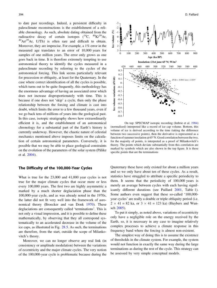
mathematically, by observing that they all correspond systematically to an accelerated decrease in the volume of the
ice caps, as illustrated in Fig. 28.5. As such, the terminations
are therefore, from the start, outside the scope of Milankovitch’s theory.
Moreover, we can no longer observe any real link (in
consistency or amplitude modulation) between the variations
of eccentricity and the major climate cycles. The very notion
of the 100,000-year cycle is problematic because during the
Quaternary these have only existed for about a million years
and so we only have about ten of these cycles. As a result,
statistics have struggled to attribute a specific periodicity to
them. It seems that the periodicity of 100,000 years is
merely an average between cycles with each having significantly different durations (see Paillard 2001, Table 1).
Some authors even suggest that these so-called ‘100,000year cycles’ are really a double or triple obliquity period (i.e.
2 Â 41 = 82 ka, or 3 Â 41 = 123 ka) (Huybers and Wunsch 2005).
To put it simply, as noted above, variations of eccentricity
only have a negligible role on the energy received by the
Earth, so, it is necessary in any case to imagine relatively
complex processes to achieve a climate response in this
frequency band where the forcing is almost non-existent.
The simplest way of doing this is to assume the existence
of thresholds in the climate system. For example, the system
would not function in exactly the same way during the large
terminations as during the rest of the cycle. This strategy can
be assessed by very simple conceptual models.
-3
-2
-1
0
1
2
3
0
100
200
300
400
500
600
700
800
900
Age (ka BP)
Ice volume (V)
dV/dt = -0.0041 inso + 2.0257
-0.8
-0.7
-0.6
-0.5
-0.4
-0.3
-0.2
-0.1
0
0.1
0.2
0.3
420 440 460 480 500 520 540 560 580 600
Insolation (21st june 65°N) W/m 2
Ice volume variations (dV/dt)
Fig. 28.5 On top: SPECMAP isotopic recording (Imbrie et al. 1984)
(normalized) interpreted like a record of ice cap volume. Bottom, this
volume of ice is derived according to the time (taking the difference
between two successive points), then the derivative is represented as a
function of summer insolation at 65°N. Good correlation between the two,
for the majority of points, is interpreted as a proof of Milankovitch’s
theory. The points which deviate substantially from this correlation are
marked by symbols which are also shown in the top figure. It is these
specific points that are the terminations
394
D. Paillard
paleoclimate reconstructions is the establishment of a reliable chronology. As such, absolute dating obtained from the
radioactive decay of certain isotopes (
14 C,
40 K/
39 Ar,
40 Ar/
39 Ar, U/Th) is often rare and difficult to obtain.
Moreover, they are imprecise. For example, a 1% error in the
measured age translates to an error of 10,000 years for
samples of one million years. The error only grows as one
goes back in time. It is therefore extremely tempting to use
astronomical theory to identify the cycles measured in a
paleoclimate recording by referring to the cycles of the
astronomical forcing. This link seems particularly relevant
for precession or obliquity, at least for the Quaternary. In the
case where correct identification of all the cycles is possible,
which turns out to be quite frequently, this methodology has
the enormous advantage of having an associated error which
does not increase disproportionately with time. This is
because if one does not ‘skip’ a cycle, then only the phase
relationship between the forcing and climate is cast into
doubt, which limits the error to a few thousand years, even if
we go back tens of millions of years into the geological past.
In this case, isotopic stratigraphy shows how extraordinarily
efficient it is, and the establishment of an astronomical
chronology for a substantial part of the Earth’s history is
currently underway. However, the chaotic nature of celestial
mechanics mentioned above imposes limits on the calculation of certain astronomical parameters. Conversely, it is
possible that we may be able to place geological constraints
on the evolution of the parameters of the solar system (Pälike
et al. 2004).
The Difficulty of the 100,000-Year Cycles
What is true for the 23,000 and 41,000 year cycles is not
true for the major climate cycles that occur more or less
every 100,000 years. The first two are highly asymmetric a
marked by a much shorter deglaciation phase than the
100,000-year cycle, and as was already noted in the 1970s,
the latter did not fit very well into the framework of asronomical theory (Broecker and van Donk 1970). These
deglaciations are consequently called ‘terminations’. This is
not only a visual impression, and it is possible to define these
mathematically, by observing that they all correspond systematically to an accelerated decrease in the volume of the
ice caps, as illustrated in Fig. 28.5. As such, the terminations
are therefore, from the start, outside the scope of Milankovitch’s theory.
Moreover, we can no longer observe any real link (in
consistency or amplitude modulation) between the variations
of eccentricity and the major climate cycles. The very notion
of the 100,000-year cycle is problematic because during the
Quaternary these have only existed for about a million years
and so we only have about ten of these cycles. As a result,
statistics have struggled to attribute a specific periodicity to
them. It seems that the periodicity of 100,000 years is
merely an average between cycles with each having significantly different durations (see Paillard 2001, Table 1).
Some authors even suggest that these so-called ‘100,000year cycles’ are really a double or triple obliquity period (i.e.
2 Â 41 = 82 ka, or 3 Â 41 = 123 ka) (Huybers and Wunsch 2005).
To put it simply, as noted above, variations of eccentricity
only have a negligible role on the energy received by the
Earth, so, it is necessary in any case to imagine relatively
complex processes to achieve a climate response in this
frequency band where the forcing is almost non-existent.
The simplest way of doing this is to assume the existence
of thresholds in the climate system. For example, the system
would not function in exactly the same way during the large
terminations as during the rest of the cycle. This strategy can
be assessed by very simple conceptual models.
-3
-2
-1
0
1
2
3
0
100
200
300
400
500
600
700
800
900
Age (ka BP)
Ice volume (V)
dV/dt = -0.0041 inso + 2.0257
-0.8
-0.7
-0.6
-0.5
-0.4
-0.3
-0.2
-0.1
0
0.1
0.2
0.3
420 440 460 480 500 520 540 560 580 600
Insolation (21st june 65°N) W/m 2
Ice volume variations (dV/dt)
Fig. 28.5 On top: SPECMAP isotopic recording (Imbrie et al. 1984)
(normalized) interpreted like a record of ice cap volume. Bottom, this
volume of ice is derived according to the time (taking the difference
between two successive points), then the derivative is represented as a
function of summer insolation at 65°N. Good correlation between the two,
for the majority of points, is interpreted as a proof of Milankovitch’s
theory. The points which deviate substantially from this correlation are
marked by symbols which are also shown in the top figure. It is these
specific points that are the terminations
394
D. Paillard