

The Successes and Difficulties
of Milankovitch’s Theory
From Hypothesis to Evidence
Milankovitch’s theory was not accepted by the majority of
geologists for a long time. In fact, stratigraphic studies by
Penk and Brückner had made it possible to define only four
successive glacial episodes in the Alps (Günz-Mindel-Riss-Würm), and not a succession of regular events. It was
not until the middle of the twentieth century that thanks to
studies on marine sediments that the number of glacial
cycles identified increased considerably (see Chap. 20, volume 1). In particular, in the 1950s, C. Emiliani carried out
the first isotopic measurements on marine carbonates,
showing more than a dozen glacial-interglacial successions
with a clear cyclicity, which put an end to the traditional
denomination (Günz-Mindel-Riss-Würm). From then on,
astronomical theory became accepted.
Emiliani thus defined the ‘isotopic stages’ which are still
used today to designate glacial and interglacial periods, odd
numbers for interglacial periods and even numbers for glacial periods. It is interesting to note that Stage 3 appears to
be an exception, since it is now unanimously considered to
be part of the last glacial period (which includes Stages 4, 3
and 2). This apparent inconsistency stems from the simple
fact that astronomical theory predicts a dominant periodicity
associated with variations in obliquity, i.e. cycles of
41,000 years.
The very rare chronological information available from
this time suggests a stage 3 around 30–50 ka BP, preceded
by many other older cycles of greater amplitude, but with
uncertain dating. It was therefore logical to begin the numbering of past interglacials from stage 3, in accordance with
the idea of a dominant cyclicity linked to the obliquity. It
was not until the 1960s and 1970s, thanks to the Pa–Th
datings, that the main cyclicity appeared to be around
100,000 years, an observation which seemed strange in the
context of astronomical theory (Broecker and van Donk
1970). This famous ‘problem of the 100,000 years’ is still a
major obstacle, as will be explained later.
Advances in dating techniques using radioisotopes have
resulted in a gradual refinement of the chronology, in particular through the use of coral reefs and magnetic reversals
that can be identified in both marine sediments and volcanic
flows. This enabled a more precise time frame to be proposed and the paleoclimate periodicities to be precisely
defined. The paper by Hays et al. (1976) identified cycles of
23,000 years, 41,000 years, and 100,000 years, which correspond well to astronomical frequencies (Berger 1978).
This demonstrated unambiguously the astronomical imprint
on the climate and the value of Milankovitch’s theory that it
is astronomy that drives the Quaternary climate cycles.
Nevertheless, this paper also highlights the main problem.
The 100,000 year cycle is the dominant cycle, but according
to the theory, it should hardly appear. It seems that there is a
link between the dominant cycle of 100,000 years and
eccentricity, but the causes are unknown. In other words, this
‘historical’ paper demonstrates both that the astronomical
theory is necessary, but that, alone, it does not explain the
observations.
A Quasi-linear System for Precession
and Obliquity
Although the astronomical periodicities are indeed present in
paleoclimate records, a simple relation connecting the two
has yet to be verified. Various analytical techniques have
been used to this end. It is thus possible to assess the consistency, in other words, the correlation in the spectral
domain (or frequency domain) between the astronomical
forcing and the paleoclimatic, geochemical and micropaleontological data. The results are quite significant for the
periodicities of 23,000 and 41,000 years, i.e. the variations
of obliquity and precession. There is therefore a close link
between astronomical changes and climate for these two
frequencies, which can be interpreted in terms of a
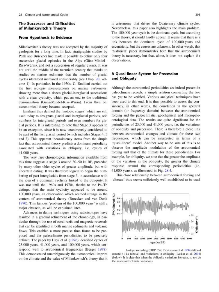
‘quasi-linear’ model. Another way to be sure of this is to
observe the amplitude modulation of the astronomical
forcing and that of the climate for these periodicities. For
example, for obliquity, we note that the greater the amplitude
of the variation in the obliquity, the greater the climate
response around the corresponding periodicities (i.e.
41,000 years), as illustrated in Fig. 28.4.
This close relationship between astronomical forcing and
‘climate’ thus seems sufficiently well established to be used
-0.4
-0.2
0
0.2
0.4
0
500 1000 1500 2000 2500 3000 3500 4000 4500 5000
22
23
24
25
Age (ka BP)
Obliquity (°)
δ 18
O filtered (‰)
Fig. 28.4 Isotope recording (ODP 659, Tiedemann et al. 1994) filtered
around 41 ka (above) and variations in obliquity (Laskar et al. 2004)
(below). It is clear that when the obliquity variations increase, so too do
the associated climate variations
28 Climate and Astronomical Cycles
393
of Milankovitch’s Theory
From Hypothesis to Evidence
Milankovitch’s theory was not accepted by the majority of
geologists for a long time. In fact, stratigraphic studies by
Penk and Brückner had made it possible to define only four
successive glacial episodes in the Alps (Günz-Mindel-Riss-Würm), and not a succession of regular events. It was
not until the middle of the twentieth century that thanks to
studies on marine sediments that the number of glacial
cycles identified increased considerably (see Chap. 20, volume 1). In particular, in the 1950s, C. Emiliani carried out
the first isotopic measurements on marine carbonates,
showing more than a dozen glacial-interglacial successions
with a clear cyclicity, which put an end to the traditional
denomination (Günz-Mindel-Riss-Würm). From then on,
astronomical theory became accepted.
Emiliani thus defined the ‘isotopic stages’ which are still
used today to designate glacial and interglacial periods, odd
numbers for interglacial periods and even numbers for glacial periods. It is interesting to note that Stage 3 appears to
be an exception, since it is now unanimously considered to
be part of the last glacial period (which includes Stages 4, 3
and 2). This apparent inconsistency stems from the simple
fact that astronomical theory predicts a dominant periodicity
associated with variations in obliquity, i.e. cycles of
41,000 years.
The very rare chronological information available from
this time suggests a stage 3 around 30–50 ka BP, preceded
by many other older cycles of greater amplitude, but with
uncertain dating. It was therefore logical to begin the numbering of past interglacials from stage 3, in accordance with
the idea of a dominant cyclicity linked to the obliquity. It
was not until the 1960s and 1970s, thanks to the Pa–Th
datings, that the main cyclicity appeared to be around
100,000 years, an observation which seemed strange in the
context of astronomical theory (Broecker and van Donk
1970). This famous ‘problem of the 100,000 years’ is still a
major obstacle, as will be explained later.
Advances in dating techniques using radioisotopes have
resulted in a gradual refinement of the chronology, in particular through the use of coral reefs and magnetic reversals
that can be identified in both marine sediments and volcanic
flows. This enabled a more precise time frame to be proposed and the paleoclimate periodicities to be precisely
defined. The paper by Hays et al. (1976) identified cycles of
23,000 years, 41,000 years, and 100,000 years, which correspond well to astronomical frequencies (Berger 1978).
This demonstrated unambiguously the astronomical imprint
on the climate and the value of Milankovitch’s theory that it
is astronomy that drives the Quaternary climate cycles.
Nevertheless, this paper also highlights the main problem.
The 100,000 year cycle is the dominant cycle, but according
to the theory, it should hardly appear. It seems that there is a
link between the dominant cycle of 100,000 years and
eccentricity, but the causes are unknown. In other words, this
‘historical’ paper demonstrates both that the astronomical
theory is necessary, but that, alone, it does not explain the
observations.
A Quasi-linear System for Precession
and Obliquity
Although the astronomical periodicities are indeed present in
paleoclimate records, a simple relation connecting the two
has yet to be verified. Various analytical techniques have
been used to this end. It is thus possible to assess the consistency, in other words, the correlation in the spectral
domain (or frequency domain) between the astronomical
forcing and the paleoclimatic, geochemical and micropaleontological data. The results are quite significant for the
periodicities of 23,000 and 41,000 years, i.e. the variations
of obliquity and precession. There is therefore a close link
between astronomical changes and climate for these two
frequencies, which can be interpreted in terms of a
‘quasi-linear’ model. Another way to be sure of this is to
observe the amplitude modulation of the astronomical
forcing and that of the climate for these periodicities. For
example, for obliquity, we note that the greater the amplitude
of the variation in the obliquity, the greater the climate
response around the corresponding periodicities (i.e.
41,000 years), as illustrated in Fig. 28.4.
This close relationship between astronomical forcing and
‘climate’ thus seems sufficiently well established to be used
-0.4
-0.2
0
0.2
0.4
0
500 1000 1500 2000 2500 3000 3500 4000 4500 5000
22
23
24
25
Age (ka BP)
Obliquity (°)
δ 18
O filtered (‰)
Fig. 28.4 Isotope recording (ODP 659, Tiedemann et al. 1994) filtered
around 41 ka (above) and variations in obliquity (Laskar et al. 2004)
(below). It is clear that when the obliquity variations increase, so too do
the associated climate variations
28 Climate and Astronomical Cycles
393