

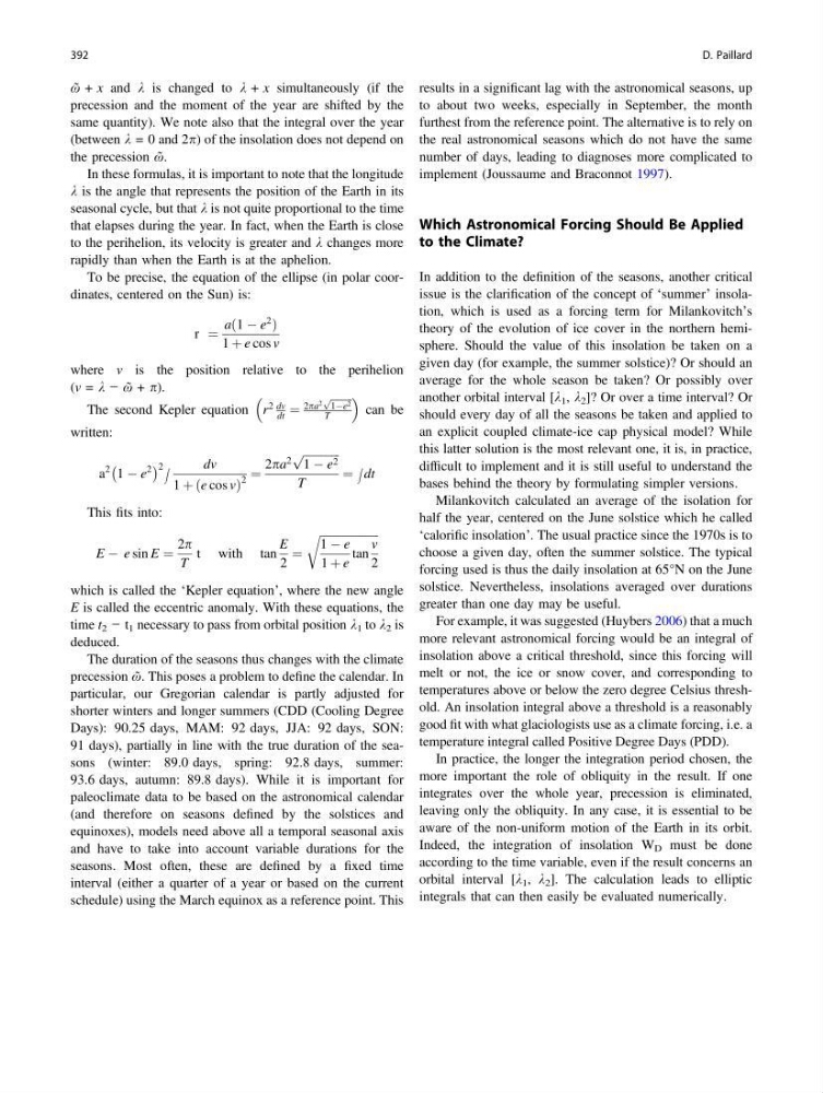
ῶ + x and k is changed to k + x simultaneously (if the
precession and the moment of the year are shifted by the
same quantity). We note also that the integral over the year
(between k = 0 and 2p) of the insolation does not depend on
the precession ῶ.
In these formulas, it is important to note that the longitude
k is the angle that represents the position of the Earth in its
seasonal cycle, but that k is not quite proportional to the time
that elapses during the year. In fact, when the Earth is close
to the perihelion, its velocity is greater and k changes more
rapidly than when the Earth is at the aphelion.
To be precise, the equation of the ellipse (in polar coordinates, centered on the Sun) is:
r ¼
a 1 À e
2
ð
Þ
1 þ e cos v
where v is the position relative to the perihelion
(v = k − ῶ + p).
The second Kepler equation r
2 dv
dt ¼
2pa
2
ffiffiffiffiffiffiffi ffi
1Àe 2
p
T
can be
written:
a
2
1 À e
2
À
Á 2Z
dv
1 þ e cos v
ð
Þ
2
¼
2pa
2
ffiffiffiffiffiffiffiffiffiffiffiffi ffi
1 À e 2
p
T
¼
Z dt
This fits into:
E À e sin E ¼
2p
T
t with tan
E
2
¼
ffiffiffiffiffiffiffiffiffiffiffiffiffiffiffiffiffiffiffiffi ffi
1 À e
1 þ e
tan
v
2
r
which is called the ‘Kepler equation’, where the new angle
E is called the eccentric anomaly. With these equations, the
time t 2 − t 1 necessary to pass from orbital position k 1 to k 2 is
deduced.
The duration of the seasons thus changes with the climate
precession ῶ. This poses a problem to define the calendar. In
particular, our Gregorian calendar is partly adjusted for
shorter winters and longer summers (CDD (Cooling Degree
Days): 90.25 days, MAM: 92 days, JJA: 92 days, SON:
91 days), partially in line with the true duration of the seasons (winter: 89.0 days, spring: 92.8 days, summer:
93.6 days, autumn: 89.8 days). While it is important for
paleoclimate data to be based on the astronomical calendar
(and therefore on seasons defined by the solstices and
equinoxes), models need above all a temporal seasonal axis
and have to take into account variable durations for the
seasons. Most often, these are defined by a fixed time
interval (either a quarter of a year or based on the current
schedule) using the March equinox as a reference point. This
results in a significant lag with the astronomical seasons, up
to about two weeks, especially in September, the month
furthest from the reference point. The alternative is to rely on
the real astronomical seasons which do not have the same
number of days, leading to diagnoses more complicated to
implement (Joussaume and Braconnot 1997).
Which Astronomical Forcing Should Be Applied
to the Climate?
In addition to the definition of the seasons, another critical
issue is the clarification of the concept of ‘summer’ insolation, which is used as a forcing term for Milankovitch’s
theory of the evolution of ice cover in the northern hemisphere. Should the value of this insolation be taken on a
given day (for example, the summer solstice)? Or should an
average for the whole season be taken? Or possibly over
another orbital interval [k 1 , k 2 ]? Or over a time interval? Or
should every day of all the seasons be taken and applied to
an explicit coupled climate-ice cap physical model? While
this latter solution is the most relevant one, it is, in practice,
difficult to implement and it is still useful to understand the
bases behind the theory by formulating simpler versions.
Milankovitch calculated an average of the isolation for
half the year, centered on the June solstice which he called
‘calorific insolation’. The usual practice since the 1970s is to
choose a given day, often the summer solstice. The typical
forcing used is thus the daily insolation at 65°N on the June
solstice. Nevertheless, insolations averaged over durations
greater than one day may be useful.
For example, it was suggested (Huybers 2006) that a much
more relevant astronomical forcing would be an integral of
insolation above a critical threshold, since this forcing will
melt or not, the ice or snow cover, and corresponding to
temperatures above or below the zero degree Celsius threshold. An insolation integral above a threshold is a reasonably
good fit with what glaciologists use as a climate forcing, i.e. a
temperature integral called Positive Degree Days (PDD).
In practice, the longer the integration period chosen, the
more important the role of obliquity in the result. If one
integrates over the whole year, precession is eliminated,
leaving only the obliquity. In any case, it is essential to be
aware of the non-uniform motion of the Earth in its orbit.
Indeed, the integration of insolation W D must be done
according to the time variable, even if the result concerns an
orbital interval [k 1 , k 2 ]. The calculation leads to elliptic
integrals that can then easily be evaluated numerically.
392
D. Paillard
precession and the moment of the year are shifted by the
same quantity). We note also that the integral over the year
(between k = 0 and 2p) of the insolation does not depend on
the precession ῶ.
In these formulas, it is important to note that the longitude
k is the angle that represents the position of the Earth in its
seasonal cycle, but that k is not quite proportional to the time
that elapses during the year. In fact, when the Earth is close
to the perihelion, its velocity is greater and k changes more
rapidly than when the Earth is at the aphelion.
To be precise, the equation of the ellipse (in polar coordinates, centered on the Sun) is:
r ¼
a 1 À e
2
ð
Þ
1 þ e cos v
where v is the position relative to the perihelion
(v = k − ῶ + p).
The second Kepler equation r
2 dv
dt ¼
2pa
2
ffiffiffiffiffiffiffi ffi
1Àe 2
p
T
can be
written:
a
2
1 À e
2
À
Á 2Z
dv
1 þ e cos v
ð
Þ
2
¼
2pa
2
ffiffiffiffiffiffiffiffiffiffiffiffi ffi
1 À e 2
p
T
¼
Z dt
This fits into:
E À e sin E ¼
2p
T
t with tan
E
2
¼
ffiffiffiffiffiffiffiffiffiffiffiffiffiffiffiffiffiffiffiffi ffi
1 À e
1 þ e
tan
v
2
r
which is called the ‘Kepler equation’, where the new angle
E is called the eccentric anomaly. With these equations, the
time t 2 − t 1 necessary to pass from orbital position k 1 to k 2 is
deduced.
The duration of the seasons thus changes with the climate
precession ῶ. This poses a problem to define the calendar. In
particular, our Gregorian calendar is partly adjusted for
shorter winters and longer summers (CDD (Cooling Degree
Days): 90.25 days, MAM: 92 days, JJA: 92 days, SON:
91 days), partially in line with the true duration of the seasons (winter: 89.0 days, spring: 92.8 days, summer:
93.6 days, autumn: 89.8 days). While it is important for
paleoclimate data to be based on the astronomical calendar
(and therefore on seasons defined by the solstices and
equinoxes), models need above all a temporal seasonal axis
and have to take into account variable durations for the
seasons. Most often, these are defined by a fixed time
interval (either a quarter of a year or based on the current
schedule) using the March equinox as a reference point. This
results in a significant lag with the astronomical seasons, up
to about two weeks, especially in September, the month
furthest from the reference point. The alternative is to rely on
the real astronomical seasons which do not have the same
number of days, leading to diagnoses more complicated to
implement (Joussaume and Braconnot 1997).
Which Astronomical Forcing Should Be Applied
to the Climate?
In addition to the definition of the seasons, another critical
issue is the clarification of the concept of ‘summer’ insolation, which is used as a forcing term for Milankovitch’s
theory of the evolution of ice cover in the northern hemisphere. Should the value of this insolation be taken on a
given day (for example, the summer solstice)? Or should an
average for the whole season be taken? Or possibly over
another orbital interval [k 1 , k 2 ]? Or over a time interval? Or
should every day of all the seasons be taken and applied to
an explicit coupled climate-ice cap physical model? While
this latter solution is the most relevant one, it is, in practice,
difficult to implement and it is still useful to understand the
bases behind the theory by formulating simpler versions.
Milankovitch calculated an average of the isolation for
half the year, centered on the June solstice which he called
‘calorific insolation’. The usual practice since the 1970s is to
choose a given day, often the summer solstice. The typical
forcing used is thus the daily insolation at 65°N on the June
solstice. Nevertheless, insolations averaged over durations
greater than one day may be useful.
For example, it was suggested (Huybers 2006) that a much
more relevant astronomical forcing would be an integral of
insolation above a critical threshold, since this forcing will
melt or not, the ice or snow cover, and corresponding to
temperatures above or below the zero degree Celsius threshold. An insolation integral above a threshold is a reasonably
good fit with what glaciologists use as a climate forcing, i.e. a
temperature integral called Positive Degree Days (PDD).
In practice, the longer the integration period chosen, the
more important the role of obliquity in the result. If one
integrates over the whole year, precession is eliminated,
leaving only the obliquity. In any case, it is essential to be
aware of the non-uniform motion of the Earth in its orbit.
Indeed, the integration of insolation W D must be done
according to the time variable, even if the result concerns an
orbital interval [k 1 , k 2 ]. The calculation leads to elliptic
integrals that can then easily be evaluated numerically.
392
D. Paillard